
Introduction
Hidden Markov Models provide a way of modeling the dynamics of sequential information. They have been used for speech recognition, part-of-speech tagging, machine translation, handwriting recognition, and, as we will see in this article, gesture recognition.
Consider a somewhat practical use-case: you are going to throw a party with a meticulously curated playlist. You would rather not let anyone have the remote as it might get lost, and letting anyone interrupt the playlist with their own selections may derail the entire event. However, you still want to give your guests the ability to control the volume and skip back and forth between tracks in the playlist. We will also assume that guests will use change tracks and control the volume responsibly.
The solution to this problem is to implement a gesture recognition system to identify simple hand motions. In this case, we only have to model 4 separate gestures: VolumeUp, VolumeDown, PrevTrack, NextTrack. Since the motions are temporal in nature, we can model each gesture using Hidden Markov Models. First, we need to cover a bit of background on what a Hidden Markov Model actually is.
Background
- First, introduce Markov Chains
- Then the Markov assumption
At the core of our problem, we want to model a distribution over a sequence of states. Consider a sequence of only 3 states \(p(x_1, x_2, x_3)\). The full computation of this can be done using the chain rule of probability:
\[ p(x_1, x_2, x_3) = p(x_1) p(x_2 | x_1) p(x_3 | x_1, x_2). \]
If the random variables of our problem are not conditionally independent, the complexity of calculating this is exponential in the number of random variables.
The Markov in Hidden Markov Models addresses this complexity. The Markov Assumption states that the probability of an event at time \(t\) is conditioned only on the previously observed event: \(p(x_t | x_{t-1})\). This is compactly represented with a graphical model, as seen in figure TODO.
TODO: Figure of basic Markov Chain
The hidden qualifier comes from the fact that the data we wish to model was generated from some underlying process that is not directly observable. A classic example for HMMs uses the weather. Imagine you had a log which had the number of water bottles a person had drank per day over the entire year. To make the problem slightly more difficult, the log entries were not associated with a date. It is reasonable to say that the amount of water a person drinks is influenced by how hot or cold it is on a particular day. So, the hidden state in this case is the weather: hot or cold. We can model this with an HMM by establishing that the amount of water (observed state) is conditioned on the weather (hidden state). Figure TODO shows this HMM graphically.
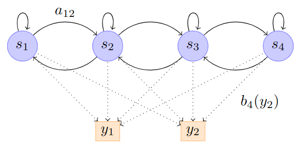
Figure 1: An HMM with 4 states and 2 observation symbols (y_1) or (y_2).
Formally, a Hidden Markov Model is defined by
- The number of hidden states \(N\).
- A transition probability matrix \(A \in \mathbb{R}^{N \times N}\), where \(a_{ij} = p(z_t = j | z_{t-1} = i)\).
- An observation symbol probability distribution \(B = \{b_j(k)\} = p(\mathbf{x}_t = k | z_t = j)\).
- An initial state distribution \(\pi_i = p(z_t = i)\).
The trainable parameters of our model are \(\lambda = (A, B, \pi)\).
Functions of an HMM
Given the basic definition of what an HMM is, how can we train the parameters defined in \(\lambda\). If we somehow already knew the parameters, how can we extract useful information from the model? Depending on our task, we can use HMMs to answer many important questions:
- Filtering computes \(p(z_t | \mathbf{x}_{1:t})\). That is, we are computing this probability as new samples come in up to time \(t\).
- Smoothing is accomplished when we have all the data in the sequence. This is expressed as \(p(z_t|\mathbf{x}_{1:T})\).
- Fixed lag smoothing allows for a trade off between accuracy and delay. It is useful in cases where we might not have the full sequence, but we wish to compute \(p(z_{t-l}|\mathbf{x}_{1:t})\) for some \(l > 0\).
- Predictions are represented as \(p(z_{t+h}|\mathbf{x}_{1:t})\), where \(h > 0\).
- MAP estimation yields the most probably state sequence \(\text{arg}\max_{\mathbf{z}_{1:T}}p(\mathbf{z}_{1:T}|\mathbf{x}_{1:T})\).
- We can sample the posterior \(p(\mathbf{z}_{1:T}|\mathbf{x}_{1:T})\).
- We can also compute \(p(\mathbf{x}_{1:T})\) by summing up over all hidden paths. This is useful for classification tasks.
Of course not all of these functions make sense for every possible task, more on that later. This article is not meant to be an exhaustive resource for all HMM functions; we will only look at the tasks necessary to train and use HMMs for isolated gesture recognition TODO: offer additional reading suggestions.
Data Processing
As far as the efficacy of our model goes, how we process the data is the most important. Our system will start with a camera that records our guests performing one of the four simple motions. For simplicity, let’s pretend that the camera has an onboard chip that detects the 2D centroids of the left hand for each frame. That helps a lot, but there is still the problem of isolating a group of frames based on when the user wanted to start and finish the command. Assuming we have a solution for both of these problems, we still need to take into account that users will gesture at different speeds. Since all of these problems are challenging in their own right, we will assume the computer vision fairy has taken care of this for us.
Each gesture in our dataset consists of 30 \((x, y)\) locations of the center of the left hand with respect to image coordinates. Even with this simplified data, we have another problem: different users may gesture from different locations. The hand locations for one user performing the VolumeUp gesture may be vastly different from another. This isn’t too bad to deal with. We could normalize or training data by subtracting the location of the hand in the first frame from the gesture. That way every input would start at \((0, 0)\). We can simplify this even further by using relative motion states.
Relative Motion States
Relative motion states discretize our data, thus simplifying the input space. The idea is quite simple: if the hand moved to the right relative to the previous frame, we assign \(x = 1\) for that frame. If it moved to the left, assign \(x = -1\). If it didn’t move at all, or did not move a significant amount, assign \(x = 0\). We apply similar rules for the \(y\) locations as well. The TODO: figure below shows the relative motion grid.
Besides greatly simplifying our input space, meaning we can use a simple categorical distribution to model these observations, we no longer have to worry about the discrepency between where each user performed the gesture.
Modeling a Gesture
Our system will consist of 4 HMM models to model the dynamics of each gesture. To determine which gesture was performed, we will given our input sequence to each one and have it compute \(p(\mathbf{x}_{1:T}; \lambda_i)\), the probability of the observation given the parameters of model \(i\). Whichever model gives the high probability wins.
TODO
- Describe EM at a high level, show the breakdown of probabilities that need to be known
- Go into forward-backwards
- Go back to EM and plug them in
Training: Expectation-Maximization
If we cannot observe the hidden states directly, how are we supposed to update the model parameters \(\lambda = (A, B, \pi)\)? We may not have all of the information, but we do have some information. We can use that to fill in the missing values with what we would expect them to be given what we already know. Then, we can update our parameters using those expected values. This is accomplished through a two-stage algorithm called Expectation-Maximization. Those familiar with k-Nearest Neighbors should already be familiar with this process.
Updating with Perfect Information
It is useful to know how we would update our parameters assuming we had perfect information. If the hidden states were fully observable, then updating our model parameters would be as straightforward as computing the maximum likelihood estimates. For \(A\) and \(\pi\), we first tally up the following counts:
\[ \hat{a}_{ij} = \frac{N_{ij}}{\sum_j N_{ij}}, \]
the number of times we expect to transition from \(i\) to \(j\) divided by the number of times we transition from \(i\) to any other state. Put simply, this computes the expected transitions from \(i\) to \(j\) normalized by all the times we expect to start in state \(i\).
For \(\pi\), we have
\[ \hat{\pi_i} = \frac{N_i}{\sum_i N_i}, \]
the number of times we expect to start in state \(i\) divided by the number of times we start in any other state.
Estimating the parameters for \(B\) depends on which distribution we are using for our observation probabilities. For a multinomial distribution, we would compute the number of times we are in state \(j\) and observe a symbol \(k\) divided by the number of times we are in state \(j\):
\[ \hat{b}_{jk} = \frac{N_{jk}}{N_k}, \]
where
\[ N_{jk} = \sum_{i=1}^N \sum_{t=1}^T \mathbb{1} (z_{i, t}=j, x_{i, t}=k). \]
It is also common to model our emission probability using a Normal distribution. We can even use a parameterized model like a neural network. TODO: provide links to examples of these
Updating with Missing Information
Now to the real problem: fill in our missing information using our observable data and the current parameter estimates. There are two important statistics that we need to compute, called the sufficient statistics.
- The expected number of transitions from \(i\) to \(j\).
- The expected number of times we are transitioning from \(i\) to any other state.
Both of these can be computed starting with the same probability conditioned on our observable data:
\[ p(z_t = i, z_{t+1} = j|\mathbf{x}_{1:T}). \]
Forwards-Backwards Algorithm
Computing joint distribution can be very computationally expensive. Fortunately for us, the Markov assumption along with operations on graphs open the door to a dynamic programming approach named the Forward-Backward algorithm.
The Forwards-Backwards Algorithm, also known as the Baum-Welch algorithm, provides an effective solution to computing the joint described above. In fact, there are many useful distributions that can be computed with this algorithm such as the filtering and smoothing tasks.
Forward Probability
The forward probability, often denoted as \(\alpha\), represents the probability of ending up at a particular hidden state \(i\) at time \(t\) having seen the observations up to that time:
\[ \alpha_t(i) = p(z_t = i, \mathbf{x}_{1:t} | \lambda). \]
This value is computed recursively starting from \(t=1\) and going forwards to \(t=T\).
Initialization
For \(t=1\), we calculate:
\[ \alpha_1(i) = \pi_i b_i(x_1),\quad 1 \leq i \leq N, \]
where \(\pi_i\) is the initial probability of state \(i\) and \(b_i(x_1)\) is the emission probability of the first observation \(x_1\) given that we are in state \(i\).
Recursion
After that, we calculate the remaining \(\alpha_t(i)\) as follows:
\[ \alpha_{t+1}(j) = b_j(x_{t+1}) \sum_{i=1}^{N} \alpha_{t}(i)a_{ij}, \]
where \(N\) is the number of hidden states, and \(a_{ij}\) is the transition probability from state \(i\) to state \(j\).
Backward Probability
The backward probability, denoted as \(\beta\), gives the probability of observing the remaining observations from time \(t+1\) to \(T\) given that we are in state \(i\) at time \(t\):
\[ \beta_t(i) = p(\mathbf{x}_{t+1:T} | z_t = i, \lambda). \]
Again, this is calculated recursively but this time starting from \(t=T\) and going backwards to \(t=1\).
Initialization
For \(t=T\), we initialize:
\[ \beta_T(i) = 1, \forall i. \]
Recursion
Then we calculate the remaining \(\beta_t(i)\) as:
\[ \beta_{t}(i) = \sum_{j=1}^{N} a_{ij}b_j(x_{t+1})\beta_{t+1}(j). \]
Calculating the Sufficient Statistics
With these two sets of probabilities, we can calculate the two required sufficient statistics as follows:
- The expected number of transitions from \(i\) to \(j\):
\[ \frac{\sum_{t=1}^{T-1} \alpha_t(i) a_{ij} b_j(x_{t+1}) \beta_{t+1}(j)}{P(X|\lambda)} \]
- The expected number of times we are transitioning from \(i\) to any other state:
\[ \frac{\sum_{t=1}^{T-1} \alpha_t(i) \beta_t(i)}{P(X|\lambda)} \]
Where \(P(X|\lambda)\) is the total probability of the observations, calculated as:
\[ P(X|\lambda) = \sum_{i=1}^{N} \alpha_T(i) \]
How does this give us \(p(z_t = i, z_{t+1} = j|\mathbf{x}_{1:T})\)?
To understand how the variables of the Forwards-Backwards algorithm relate to the original probabilities, we can express the term \(p(z_t = i, z_{t+1} = j|\mathbf{x}_{1:T})\) in terms of the original probability distributions in the HMM:
- \(\pi_i\) - the probability of starting in state \(i\),
- \(a_{ij}\) - the probability of transitioning from state \(i\) to state \(j\),
- \(b_j(x_t)\) - the probability that state \(j\) will emit observation \(x_t\).
The joint probability \(p(z_t = i, z_{t+1} = j, \mathbf{x}_{1:T})\) would represent the probability of being in state \(i\) at time \(t\), moving to state \(j\) at time \(t+1\), and observing the sequence of emissions \(\mathbf{x}_{1:T}\). This can be factored as follows due to the Markov property:
\[ p(z_t = i, z_{t+1} = j, \mathbf{x}_{1:T}) = p(\mathbf{x}_{1:t}, z_t = i)p(z_{t+1} = j| z_t = i)p(\mathbf{x}_{t+1:T} | z_{t+1} = j, \mathbf{x}_{1:t}). \]
Using our definitions of \(\alpha\) and \(\beta\), we can rewrite this in terms of our HMM quantities:
\[ p(z_t = i, z_{t+1} = j, \mathbf{x}_{1:T}) = \alpha_t(i)a_{ij}b_j(x_{t+1})\beta_{t+1}(j). \]
Here, \(\alpha_t(i)\) represents \(p(\mathbf{x}_{1:t}, z_t = i)\), the joint probability of the observations until time \(t\) and being in state \(i\) at time \(t\), and \(\beta_{t+1}(j)\) represents \(p(\mathbf{x}_{t+1:T} | z_{t+1} = j)\), the probability of the observations from time \(t+1\) to \(T\) given we’re in state \(j\) at time \(t+1\).
Then, to obtain \(p(z_t = i, z_{t+1} = j|\mathbf{x}_{1:T})\), we divide by \(p(\mathbf{x}_{1:T})\) to normalize the probabilities, which is the sum over all states of \(\alpha_T(i)\), or equivalently, the sum over all states of \(\beta_1(i)\pi_i b_i(x_1)\).
This gives us:
\[ p(z_t = i, z_{t+1} = j|\mathbf{x}_{1:T}) = \frac{\alpha_t(i)a_{ij}b_j(x_{t+1})\beta_{t+1}(j)}{\sum_{i=1}^{N}\alpha_T(i)}. \]
This is the same expression as before, but broken down in terms of the original HMM quantities and the forward and backward variables. This can also be explained through graph properties and operations. See Sargur Srihari’s excellent lecture slides for more details.