Active Contours
Resources
Introduction
Snakes, as named by Kass et al., is a spline curve that is minimized such that it moves towards distinct image features such as edges. The closed curve, or snake, can be thought of as a rubber band.
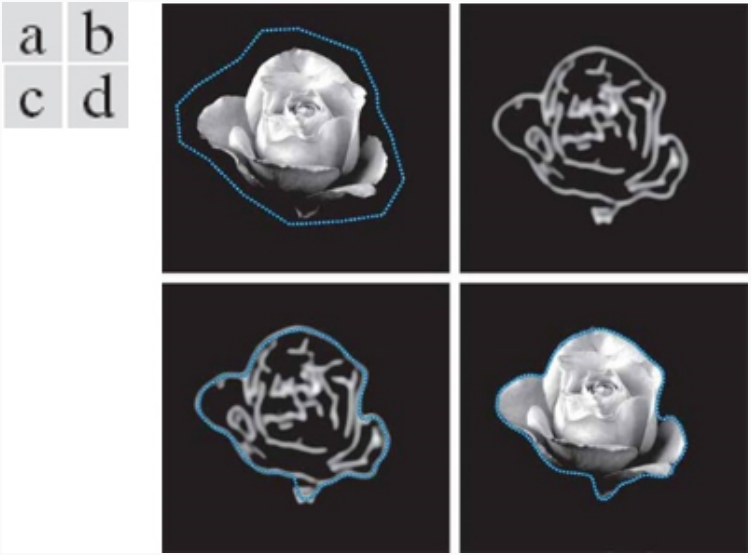
Figure 1: Example of snake snapping to object. (Copyright 2018, 2008 Pearson Education, Inc.)
When stretched out, the band has an internal potential energy that forces the band to close in around some rigid object which exerts force against the band’s internal energy. This method does not tout itself it be a fully autonomous way to segment interesting features. Instead, it is useful in semi-supervised settings where the user knows a general region of interest. The minimization of the snake will segment the desired object under reasonable settings.
Parametric Representation
The contour is represented as a curve using a parametric representation:
\[ (x, y) = (g(s), h(s)). \]
The argument \(s\) can be thought of as the trajectory of the curve.
Parametric representations are a natural choice for representing curves in computing due to their compact representation. For example, a circle is defined by \(x^2 + y^2 = r^2\). The individual values \(x\) and \(y\) are
\begin{align*} x &= r\cos(s)\\ y &= r\sin(s) \end{align*}
It can then be shown that
\begin{align*} x^2 + y^2 &= r^2\cos^2(s) + r^2\sin^2(s)\\ &= r^2\big(\cos^2(s) + \sin^2(s)\big)\\ &= r^2. \end{align*}
As a vector, we can represent \((x, y)\) as
\begin{equation*} \mathbf{c}= \begin{bmatrix} x\\ y \end{bmatrix}= \begin{bmatrix} x\\ \pm \sqrt{r^2 - x^2} \end{bmatrix}. \end{equation*}
Using the more efficient parametric representation, this vector is defined as
\begin{equation*} \mathbf{c}= \begin{bmatrix} r\cos(s)\\ r\sin(s) \end{bmatrix}. \end{equation*}
Another example using parametric representation is that of spline curves.
\begin{align*} x(t) &= a_xt^3 + b_xt^2 + c_xt + dx\\ y(t) &= a_yt^3 + b_yt^2 + c_yt + dy \end{align*}
Then, \(\mathbf{f}(t) = (x(t), y(t))\).
Motivation of the Fundamental Snake Equation
Given a vector \(\mathbf{c}(s) = \big(x(s), y(s)\big)\) normalized such that \(0 \leq s \leq 1\), an energy function is defined based on internal and external forces:
\[ E(\mathbf{c}) = E_{int} + E_{ext}. \]
As the snake is updated iteratively, its final position should be one such that the energy \(E\) is minimized.
The internal energy function is given as
\[ E_{int} = \frac{\alpha}{2}\|\mathbf{c}’(s)\|^2 + \frac{\beta}{2}\|\mathbf{c}’’(s)\|^2, \]
where the first-order term is controlled by \(\alpha\) and the second-order term controlled by \(\beta\). The first-order term gives the snake an elastic quality that shrinks towards a rigid object. The second-order term controls the siffness of the contour.
External Force
The external force \(E_{ext}\) is based on the magnitude of the image gradient:
\[ E_{img}(x, y) = \|\nabla f(x, y)\|^2. \]
Additionally, the gradient vectors are recorded. The combination of the two serve to represent a force field of the edge map.
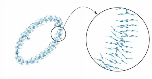
Figure 2: Force field using the edge map using normalized gradients. Source: Pearson Education, Inc.
Energy Minimization
The total energy of the snake is then
\[ E(\mathbf{c}(s)) = \int_0^1 \frac{\alpha}{2}\|\mathbf{c}’(s)\|^2 ds + \int_0^1 \frac{\beta}{2}\|\mathbf{c}’’(s)\|^2 ds + \int_0^1 E_{img}(\mathbf{c}(s))ds. \]
To find the minimum energy, we write the above equation as a function \(F\) and take its derivative with respect to s. The minimum energy must satisfy
\[ \frac{\partial}{\partial s}\Big(\frac{\partial F}{\partial\mathbf{c}’}\Big) - \frac{\partial^2}{\partial s^2} \Big(\frac{\partial F}{\partial \mathbf{c}’’}\Big) - \frac{\partial F}{\partial \mathbf{c}} = 0. \]
Solving for the partials above yields
\[ \alpha \mathbf{c}’’ - \beta \mathbf{c}’’’’ - \nabla E_{img} = 0. \]
Since the derivative of energy is a force, and the external force of the object is against the internal force of the snake, we can write
\[ \nabla E_{img} = -\mathbf{F}. \]
Under this perspective, the minimum energy is found when
\[ \alpha \mathbf{c}’’(s) - \beta \mathbf{c}’’’’(s) + \mathbf{F}(\mathbf{c}(s)) = 0. \]
Iterative Solution
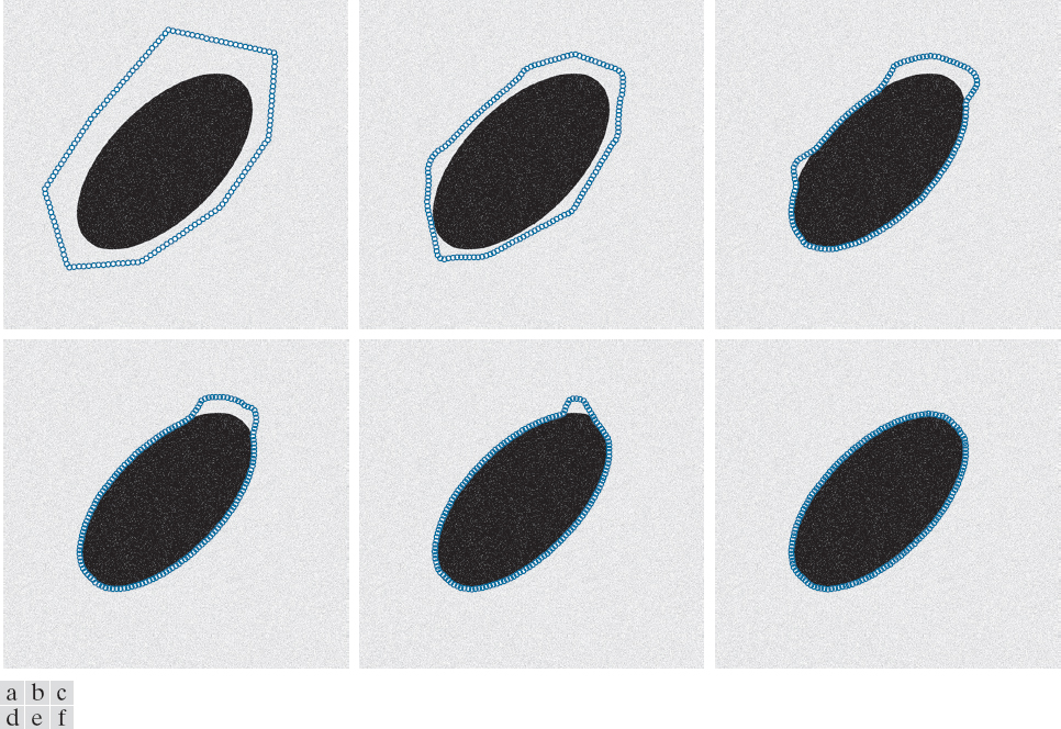
Figure 3: From top left to bottom right: initial snake, 10 steps, 50, 100, 150, 200. Source: Pearson Education, Inc.
To solve this as an iterative process over time \(t\), we write the force vector \(\mathbf{F}\) in terms of its 2D components dependent on \(t\):
\[ \mathbf{F}(\mathbf{c}(s, t)) = \mathbf{F}(x(s, t), y(s, t)) = \begin{bmatrix} F_x (x(s, t), y(s, t))\\ F_y (x(s, t), y(s, t)) \end{bmatrix}. \]
For the internal energy components, we take the partial derivative of \(\mathbf{c}\) with respect to time:
\[ \frac{\partial \mathbf{c}(s, t)}{\partial t} = \begin{bmatrix} \frac{\partial x(s, t)}{\partial t}\\ \frac{\partial y(s, t)}{\partial t}\\ \end{bmatrix}. \]
These derivatives rely on second and fourth order derivatives. For \(x(s, t)\), this is
\[ \frac{\partial x(s, t)}{\partial t} = \alpha \frac{\partial^2 x(s, t)}{\partial s^2} - \beta \frac{\partial^4 x(s, t)}{\partial s^4} + F_x(x(s, t), y(s, t)). \]
The partial for \(y\) follows a similar formulation. These derivatives are approximated using finite differences. The second order derivative is approximated as
\[ \frac{\partial^2 x(s, t)}{\partial s^2} = x’’(k, t) = x(k + 1, t) - 2x(k, t) + x(k-1, t), \]
and the fourth order derivative is approximated as
\[ \frac{\partial^4 x(s, t)}{\partial s^4} = x’’’’(k, t) = x(k + 2, t) - 4x(k + 1, t) + 6x(k, t) - 4x(k-1, t) + x(k-2, t). \]
The finite differences can be written in matrix form as a pentadiagonal banded matrix. Adding back the external force yields a much simpler equation:
\[ Dx + F_x(\mathbf{x}(t), \mathbf{y}(t)) = 0, \]
where
\[ D = \alpha D_2 - \beta D_4, \]
the matrix of finite differences.
Solving the above equation involves taking a finite step in time multiplied by the product of the negative time derivatives. To simplify this process further, an assumption is made that the external force remains constant over time.
\[ D\mathbf{x}(t) + \mathbf{F}_x(\mathbf{x}(t-1, \mathbf{y}(y-1)) = -\gamma(\mathbf{x}(t) - \mathbf{x}(t-1)) \]
This is solved using matrix inversion yielding the final update for time \(t\) as
\[ \mathbf{x}(t) = A[\mathbf{x}(t-1) + \gamma \mathbf{F}_x(\mathbf{x}(t-1), \mathbf{y}(t-1))], \]
where \(A = [I - D]^{-1}\).
The step for \(\mathbf{y}(t)\) follows a similar formulation.
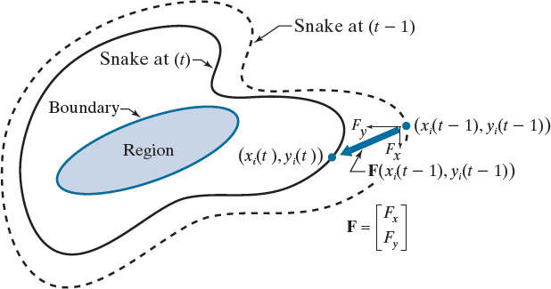
Figure 4: Snake transition between time steps. Source: Pearson Education, Inc.
Applications
In the original paper, the authors show an application where an initial frame of video is initialize with a snak by hand to track the contours of a mouth. From that point, the shape automatically matches the subsequent frames.
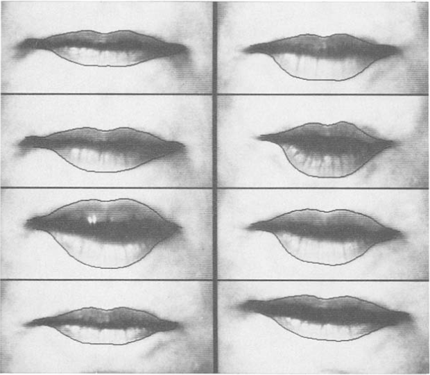
Figure 5: Snakes for motion tracking (Kass et al.)