All-Pairs Shortest Paths
The slides accompanying these notes can be found here.
TychoLink is a telecommunications company looking to optimize its network for the fastest and most efficient data transfer possible. The network consists of multiple routers, each connected by various types of links that differ in latency and bandwidth. The company wants to ensure that data packets can travel from any router to any other router in the network using the path that offers the best balance between low latency and high bandwidth. There are three objectives in total:
- Determine the all-pairs shortest paths across the network, taking into account both latency and bandwidth.
- Minimize the overall latency for data packet transmission across the network.
- Maximize the effective bandwidth along the chosen paths to ensure high data transfer rates.
Given the solutions discussed in Single-Source Shortest Paths, we can simply run the Bellman-Ford algorithm for each router in the network to find the shortest paths to all other routers. This results in a time complexity of \(O(V^2 E)\). If the network is dense, then the number of edges \(E = \Theta(V^2)\), which results in a time complexity of \(O(V^4)\).
These notes discuss another solution, the Floyd-Warshall algorithm, which can find the shortest paths between all pairs of routers in the network in \(O(V^3)\) time. The algorithm is particularly useful when the network is dense, as it is more efficient than running the Bellman-Ford algorithm for each router.
Problem Representation
Given a network \(G = (V, E)\) and a set of weights \(W = (w_{ij})\) for each edge \((i, j) \in E\), the goal is to find the shortest path between all pairs of vertices in \(V\). The graph and weights will be represented as an adjacency matrix with entries \(w_{ij}\) for each edge \((i, j) \in E\).
\[ w_{ij} = \begin{cases} 0 & \text{if } i = j \\ \text{weight of edge } (i, j) & \text{if } i \neq j, (i, j) \in E \\ \infty & \text{if } i \neq j, (i, j) \notin E. \end{cases} \]
The \((i, j)\) entry of the output matrix is \(\delta(i, j)\), the shortest-path weight from \(i\) to \(j\).
A Naive Solution
To construct a dynamic programming solution, we need to establish that the problem has optimal substructure. The shortest path structure was first discussed in Single-Source Shortest Paths.
Recursive Solution
Step 2 is to state the recursive solution. Let \(l_{ij}^{( r)}\) be the minimum weight of any path \(i \leadsto j\) that contains at most \(r\) edges. For \(r = 0\), the cost is either 0 if \(i = j\) or \(\infty\) otherwise.
For \(r = 1\), try all possible predecessors \(k\) of \(j\).
\begin{align*} l_{ij}^{( r)} &= \min \Big\{l_{ij}^{(r-1)}, \min \{l_{ik}^{(r-1)} + w_{kj} : 1 \leq k \leq n\}\Big\}\\ &= \min \{l_{ik}^{(r-1)} + w_{kj} : 1 \leq k \leq n\}. \end{align*}
Either the solution comes from a path of length \(r-1\) or from a path of length \(r-1\) with an additional edge \((k, j)\). The shortest path weights \(\delta(i, j)\) contain at most \(n-1\) edges since the shortest path cannot contain a cycle. This implies that \(\delta(i, j) = l_{ij}^{(n-1)} = l_{ij}^{(n)} = l_{ij}^{(n+1)} = \ldots\)
Bottom-Up Approach
Starting with a matrix \(W = (w_{ij})\), where \(w_{ij}\) are the edge weights, the following approach computes a series of matrices \(L^{(0)}, L^{(1)}, \ldots, L^{(n-1)}\), where \(L^{( r)} = (l_{ij}^{( r)})\). The final matrix \(L^{(n-1)}\) contains the shortest path weights.
def extend_shortest_paths(L, W):
    n = len(L)
    L_prime = [[float('inf') for _ in range(n)] for _ in range(n)]
    for i in range(n):
        for j in range(n):
            for k in range(n):
                L_prime[i][j] = min(L_prime[i][j], L[i][k] + W[k][j])
    return L_prime
This function has the structure of matrix multiplication and has a running time of \(O(n^3)\). Since this must be repeated \(n\) times, the total running time is \(O(n^4)\).
Since they are so similar, we can actually reframe this as matrix multiplication. This will lead to a more efficient algorithm. Start with the statement being computed inside the loop:
\[ l_{ij}^{( r)} = \min \{l_{ij}^{( r)}, l_{ik}^{(r-1)} + w_{kj}\}. \]
If we swap \(\min\) with \(+\) and \(\cdot\) with \(\min\), we can rewrite this as a matrix multiplication:
\[ l_{ij}^{( r)} = l_{ij}^{( r)} + l_{ik}^{(r-1)} \cdot w_{kj}. \]
For this to yield the correct result, we also need to swap the identity of \(\min\), which is \(\infty\), with the identity of \(+\), which is 0.
Faster APSP
What’s the point?
The purpose of this reframing is to benefit from the associative property of matrix multiplication. As it turns out, our modified matrix multiplication using \(\min\) is also associative. This allows us to compute the shortest paths in \(O(n^3 \lg n)\) time. Consider that we only really care about \(L^{(n-1)}\). If we are not using negative weights, then computing anything above \(n-1\) will yield the same result.
We can get to this result in fewer steps by using repeated squaring.
\begin{align*} L^{(1)} &= &W, &\quad\\ L^{(2)} &= &W^2 &= W \cdot W,\\ L^{(4)} &= &W^4 &= W^2 \cdot W^2,\\ & &\vdots &\\ L^{(2^{\lceil \lg (n-1) \rceil})} &= &W^{2^{\lceil \lg (n-1) \rceil}} &= W^{2^{\lceil \lg (n-1) \rceil - 1}} \cdot W^{2^{\lceil \lg (n-1) \rceil - 1}}. \end{align*}
In total, we compute \(O(\lg n)\) matrices, each of which takes \(O(n^3)\) time to compute. The total running time is \(O(n^3 \lg n)\).
def faster_all_pairs_shortest_paths(W):
    n = len(W)
    L = W
    m = 1
    while m < n - 1:
        L = extend_shortest_paths(L, L)
        m *= 2
    return L
Since we know that \(L^{( r)} = L^{(n-1)}\) for all \(r \geq n-1\), we can stop the loop when \(m \geq n-1\).
Example
Exercise 23.1-1: Run APSP on the following graph and show the resulting matrices at each step.
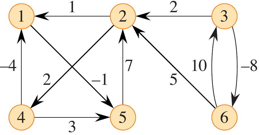
Figure 1: Figure 23.2 from (Cormen et al. 2022).
The Floyd-Warshall Algorithm
The next solution to the APSP problem is the Floyd-Warshall algorithm. This algorithm can handle negative weight edges, but it will fail to produce a result if a negative weight cycle exists. It is a dynamic programming approach that reconsiders the structure of a shortest path.
Given a path \(p = \langle v_1, v_2, \dots, v_l\rangle\), an intermediate vertex is an vertex of \(p\) other than \(v_1\) and \(v_l\). Then define \(d_{ij}^{(k)}\) as the weight of the shortest path from \(i\) to \(j\) that uses only the vertices \(\{1, 2, \dots, k\}\) as intermediate vertices. Note that the vertices are arbitrarily numbered from 1 to \(n\).
Consider a shortest path \(i \leadsto j\) that uses intermediate vertices in the set \(\{1, 2, \dots, k\}\):
- Drop \(k\): If \(k\) is not an intermediate vertex, then the path is a shortest path from \(i\) to \(j\) that uses only the vertices \(\{1, 2, \dots, k-1\}\) as intermediate vertices.
- Split \(k\): If \(k\) is an intermediate vertex, split the path \(p\) into \(i \overset{p_1}{\leadsto} k \overset{p_2}{\leadsto} j\). In this case, \(p_1\) is a shortest path from \(i\) to \(k\) that uses only the vertices \(\{1, 2, \dots, k-1\}\) as intermediate vertices, and \(p_2\) is a shortest path from \(k\) to \(j\) that uses only the vertices \(\{1, 2, \dots, k-1\}\) as intermediate vertices.
Notice that, in either case, the set of intermediate vertices is reduced.
Recursive Solution
Let \(d_{ij}^{(k)}\) be the weight of a shortest path from \(i\) to \(j\) that uses only the vertices \(\{1, 2, \dots, k\}\) as intermediate vertices. The base case is \(d_{ij}^{(0)} = w_{ij}\).
\[ d_{ij}^{(k)} = \begin{cases} w_{ij} & \text{if } k = 0,\\ \min \{d_{ij}^{(k-1)}, d_{ik}^{(k-1)} + d_{kj}^{(k-1)}\} & \text{if } k \geq 1. \end{cases} \]
The goal is to compute \(D^{(n)} = (d_{ij}^{(n)})\), since all intermediate vertices belong to the set \(\{1, 2, \dots, n\}\).
Bottom-Up Approach
With a recurrent solution in hand, a bottom-up approach can be used to compute the shortest path. The Floyd-Warshall algorithm takes as input a weighted adjacency matrix \(W = (w_{ij})\) and returns a matrix \(D = (d_{ij})\).
def floyd_warshall(W):
    n = len(W)
    D = W
    for k in range(n):
        D_prime = [[float('inf') for _ in range(n)] for _ in range(n)]
        for i in range(n):
            for j in range(n):
                D_prime[i][j] = min(D[i][j], D[i][k] + D[k][j])
        D = D_prime
    return D
This provides a running time of \(\Theta(n^3)\).
Constructing the Shortest Paths
The Floyd-Warshall algorithm can be modified to construct the shortest paths themselves. This can be done by maintaining a matrix \(P\) that stores the predecessor of each vertex along the shortest path. Let \(P^{(k)} = (p_{ij}^{(k)})\) for \(k = 0, 1, \dots, n\) be the matrix of predecessors. Each entry \(p_{ij}^{(k)}\) is defined recursively. The base case is
\[ p_{ij}^{(0)} = \begin{cases} i & \text{if } i \neq j \text{ and } w_{ij} < \infty,\\ \text{NIL} & \text{otherwise}. \end{cases} \]
The recursive case is
\[ p_{ij}^{(k)} = \begin{cases} p_{kj}^{(k-1)} & \text{if } d_{ij}^{(k-1)} > d_{ik}^{(k-1)} + d_{kj}^{(k-1)},\\ p_{ij}^{(k-1)} & \text{otherwise}. \end{cases} \]
In words, the recursive case is split into two parts. If the shortest path from \(i\) to \(j\) has \(k\) as an intermediate vertex, then it is \(i \leadsto k \leadsto j\) where \(k \neq j\). In this case, choose \(j\)’s predecessor to be the predecessor of \(j\) on a shortest path from \(k\) to \(j\) with all intermediate vertices less than \(k\): \(p_{ij}^{(k)} = p_{kj}^{(k-1)}\).
The second subcase is when \(k\) is not an intermediate vertex. Keep the same predecessor as the shortest path from \(i\) to \(j\) with all intermediate vertices less than \(k\): \(p_{ij}^{(k)} = p_{ij}^{(k-1)}\).
Example
Walk through the Floyd-Warshall algorithm on the graph from the previous example. A Python notebook of this example is available in the repository.
Transitive Closure of a Graph
The algorithms presented above successfully solve the all-pairs shortest paths problem. What if we simply wanted to determine if a path exists between for all pairs of vertices? The answer to this question lies in the transitive closure of a graph.
Let \(G = (V, E)\) be a directed graph with a vertex set \(V = \{1, 2, \dots, n\}\). The transitive closure of \(G\) is a graph \(G^* = (V, E^*)\) such that \((i, j) \in E^*\) if there is a path from \(i\) to \(j\) in \(G\).
One solution to this problem is to assign a weight of 1 to each edge of \(E\) and run the Floyd-Warshall algorithm. If \(d_{ij} < n\), then there is a path from \(i\) to \(j\) in \(G\). If \(d_{ij} = \infty\), then there is no path from \(i\) to \(j\) in \(G\). First, substitute the \(\min\) and \(+\) operations with \(\lor\) (OR) and \(\land\) (AND), respectively. This will allow us to determine if a path exists between two vertices.
Just like Floyd-Warshall, we will maintain a series of matrices \(T^{(0)}, T^{(1)}, \ldots, T^{(n-1)}\), where \(T^{( r)} = (t_{ij}^{( r)})\). The final matrix \(T^{(n)}\) contains the transitive closure of the graph. The values are defined as
\[ t_{ij}^{( r)} = \begin{cases} 1 & \text{if } r = 0 \text{ and } (i, j) \in E,\\ 1 & \text{if } r > 0 \text{ and } (t_{ij}^{(r-1)} = 1 \lor (t_{ik}^{(r-1)} \land t_{kj}^{(r-1)})),\\ 0 & \text{otherwise}. \end{cases} \]
def transitive_closure(W):
    n = len(W)
    T = W
    for k in range(n):
        T_prime = [[0 for _ in range(n)] for _ in range(n)]
        for i in range(n):
            for j in range(n):
                T_prime[i][j] = T[i][j] or (T[i][k] and T[k][j])
        T = T_prime
    return T
This algorithm has a running time of \(\Theta(n^3)\) while using simpler operations compared to the Floyd-Warshall algorithm.