Binary Search Trees
The slides for these lecture notes are available here.
A $n$-ary tree is a graph-based data structure in which each node has up to \(n\) subnodes. It is supported by the following operations (not exclusive):
- Search
- Insert
- Delete
Tree-based data structures are defined by the following properties.
- The size of a tree \(T\) is determined by the total number of nodes in \(T\).
- The root of a tree \(T\) is the starting point of \(T\).
- A leaf node of a tree \(T\) is a node that has no sub-nodes.
- The height of a tree is determined by the length of the shortest path between the root of \(T\) and the lowest leaf node of \(T\).
If we limit the number of subnodes each node may have to 2, the structure becomes known as a binary tree. Limiting the structure in this way is of interest to us because of the efficiency benefits seen in operations applied to binary trees. If we narrow the scope of these trees further, we can define a binary search tree whose search operation, as the name might suggest, runs in \(\Theta(lg n)\) worst-case time.
Binary Search Trees
A binary search tree is a regular binary tree with references to the left, right, and parent nodes, defined by the following property:
Let \(x\) be a node in a binary search tree. If \(y\) is a node in the left subtree of \(x\), then \(y.key \leq x.key\). If \(y\) is a node in the right subtree of \(x\), then \(y.key \geq x.key\).
Under this definition, operations such as search, insert, and delete can be performed in \(\Theta(lg n)\) worst-case time assuming that the tree is balanced. Later, we will explore a variant of the binary search tree that guarantees a balanced tree.
A tree node implemented in Python might look like this:
class Node:
    def __init__(self, key):
        self.key = key
        self.left = None
        self.right = None
        self.parent = None
Operations
Traversals
Like any other graph-based structure, a tree can be traversed using either depth-first or breadth-first search. Only an inorder depth-first search is of interest for a binary search tree, as we will see below. Consider the given tree in the figure below. Performing an inorder traversal on this tree yields the keys in sorted order from smallest to largest.
def inorder_tree_walk(x):
    if x is not None:
        inorder_tree_walk(x.left)
        print(x.key)
        inorder_tree_walk(x.right)
Traversing the entire tree takes \(\Theta(n)\) time, as each node must be visited once. Searching a tree, however, only takes \(\Theta(lg n)\) time. The search algorithm is defined recursively as follows:
def tree_search(x, k):
    if x is None or k == x.key:
        return x
    if k < x.key:
        return tree_search(x.left, k)
    else:
        return tree_search(x.right, k)
Consider the balanced tree shown in the figure below. If we search for the key 15, notice that after the first comparison with the root, the search space goes from 15 nodes to 7 nodes. After the second comparison, the search space goes from 7 nodes to 3 nodes. After the third comparison, the search space goes from 3 nodes to 1 node. This is the essence of binary search, and it is why the search operation runs in \(\Theta(lg n)\) time.
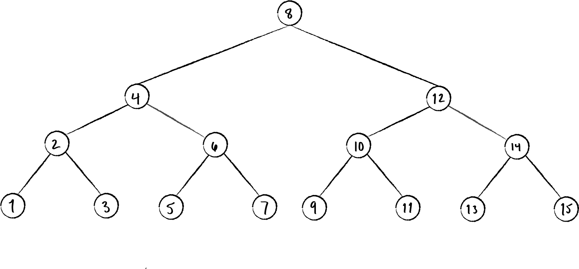
Figure 1: A balanced binary search tree
Minimum
In a BST, the minimum value is the leftmost node. Finding the minimum is as easy as traversing down the left branch until a leaf node is reached.
def tree_minimum(x):
    while x.left is not None:
        x = x.left
    return x
Maximum
In a BST, the maximum value is the rightmost node. Finding the maximum is as easy as traversing down the right branch until a leaf node is reached.
def tree_maximum(x):
    while x.right is not None:
        x = x.right
    return x
Successor
The successor and predecessor operations are useful for the delete operation defined below. The successor of a node \(x\) is the node with the smallest key greater than \(x.key\). If \(x\) has a right subtree, then the successor of \(x\) is the minimum of the right subtree. If \(x\) has no right subtree, then the successor of \(x\) is the lowest ancestor of \(x\) whose left child is also an ancestor of \(x\).
def tree_successor(x):
    if x.right is not None:
        return tree_minimum(x.right)
    y = x.parent
    while y is not None and x == y.right:
        x = y
        y = y.parent
    return y
Predecessor
The predecessor of a node \(x\) is the node with the largest key less than \(x.key\). If \(x\) has a left subtree, then the predecessor of \(x\) is the maximum of the left subtree. If \(x\) has no left subtree, then the predecessor of \(x\) is the lowest ancestor of \(x\) whose right child is also an ancestor of \(x\).
def tree_predecessor(x):
    if x.left is not None:
        return tree_maximum(x.left)
    y = x.parent
    while y is not None and x == y.left:
        x = y
        y = y.parent
    return y
Insert
Inserting an item into a binary search tree follows the same logic as traversal. Starting at the root, the key is compared to see if it is greater than the root’s key. If so, recursively traverse down the right branch. If not, recursively traverse down the left branch. This process continues until a leaf node is reached, at which point the new node is inserted as a child of the leaf node.
This process will not necessarily result in a balanced tree. In fact, if the keys are inserted in sorted order, the tree will be a linked list. This is the worst-case scenario for a binary search tree, as the search operation will then run in \(\Theta(n)\) time.
The full algorithm is given below.
def tree_insert(T, z):
    y = None
    x = T.root
    while x is not None:
        y = x
        if z.key < x.key:
            x = x.left
        else:
            x = x.right
    z.parent = y
    if y is None:
        T.root = z
    elif z.key < y.key:
        y.left = z
    else:
        y.right = z
Delete
Deleting a node is not a straightforward as insert. Depending on the structure of the subtree, one of three cases must be considered.
- If \(z\) has no subnodes, simply remove \(z\) from the tree.
- If \(z\) has one subnode, replace \(z\) with its subnode.
- If \(z\) has two subnodes, replace \(z\) with its successor. It is a bit more complicated than this, as we explore below.
In case 3, node \(z\) has both a left and right subnode. The first step is to find the successor of \(z\), \(y\). Since \(z\) has 2 subnodes, its successor has no left subnode (convince yourself of this). Likewise, its predecessor has no right subnode. If \(y\) is the right subnode of \(z\), replace \(z\) by \(y\).
If \(y\) is not the right subnode of \(z\), it is somewhere further down the right branch. In this case, replace \(y\) by its right subnode before replacing \(z\) by \(y\). The figure below shows the removal of node 12 from the tree in the figure above.
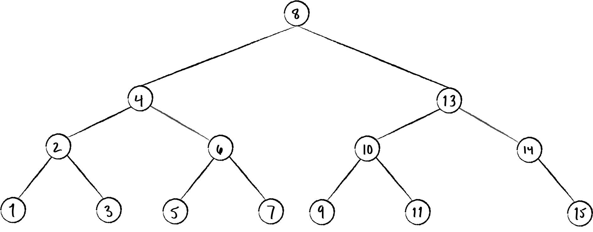
Figure 2: Deleting node 12 from the tree
Even though only 1 node was moved (13 to 12’s old position), the process of deleting a node actually involves transplanting a subtree to a new position. This is defined algorithmically as follows:
def transplant(T, u, v):
    if u.parent is None:
        T.root = v
    elif u == u.parent.left:
        u.parent.left = v
    else:
        u.parent.right = v
    if v is not None:
        v.parent = u.parent
In the code above, u is the node to be replaced, and v is the node to replace it. Updating v’s left and right subnodes are done in the calling function tree_delete, as seen below.
def tree_delete(T, z):
    if z.left is None:  # Case 1 and 2
        transplant(T, z, z.right)
    elif z.right is None: # Also case 1 and 2
        transplant(T, z, z.left)
    else: # Case 3
        y = tree_minimum(z.right) # get successor
        if y != z.right:
            transplant(T, y, y.right)
            y.right = z.right
            y.right.parent = y
        transplant(T, z, y)
        y.left = z.left
        y.left.parent = y
Analysis
Insert, delete, and search all run in \(\Theta(h)\) time, where \(h\) is the height of the tree. If the tree is balanced, \(h = \Theta(lg n)\), and all operations run in \(\Theta(lg n)\) time. If the tree is not balanced, \(h = \Theta(n)\), and all operations run in \(\Theta(n)\) time.