Camera Models
Reading
- Chapters 1 and 7 (Forsyth and Ponce)
- https://www.scratchapixel.com/
- https://docs.google.com/presentation/d/1RMyNQR9jGdJm64FCiuvoyJiL6r3H18jeNIyocIO9sfA/edit#slide=id.p
- http://vision.stanford.edu/teaching/cs131_fall1617/lectures/lecture8_camera_models_cs131_2016.pdf
- http://vlm1.uta.edu/~athitsos/courses/cse4310_spring2021/lectures/11_geometry.pdf
Outline
- Pinhole model
- Coordinates of a pinhole model
- Perspective projections
- Homogeneous coordinates
- Computer graphics perspective
- Lenses
- Intrinsic and extrensic parameters
- From world to camera to image space
- Camera calibration
Pinhole Model
Imagine piercing a small hole into a plate and placing it in front of a black screen. The light that enters through the pinhole will show an inverted image against the back plane. If we place a virtual screen in front of the pinhole plate, we can project the image onto it. This is the basic idea behind a pinhole camera model.
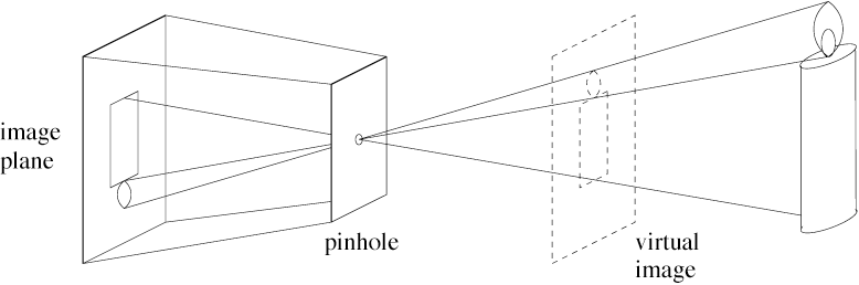
Figure 1: Pinhole camera model (Forsyth and Ponce).
Virtual Camera Coordinates
There are two sets of coordinates for each object in the pinhole camera model. First are the actual coordinates of the visible points as seen from the camera. For real images, these points are continuous. For virtual images, these are discrete. To produce an actual image, a set of 3D coordinates are projected onto the image plane. These 3D coordinates are with respect to the camera’s coordinate system.
We can represent the transformation from camera coordinates to image coordinates with a projection matrix. There are many properties of the camera that must be considered, such as the lens, resolution, etc. We will start with a simple projection matrix.
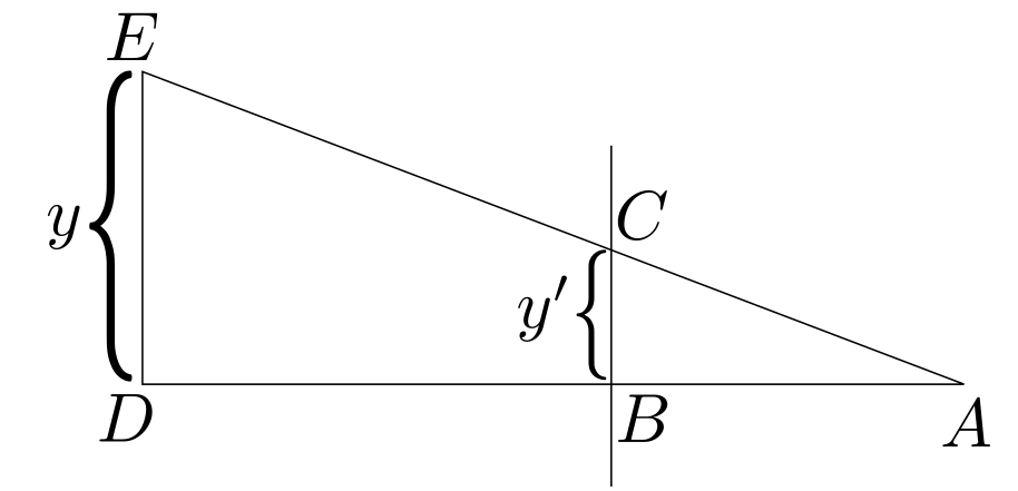
Figure 2: Derivation of simple perspective projection.
In the figure above, the camera is located at point \(A\) with its viewing plane defined by \(BC\). The \(y\) value of the world space coordinate is given by \(DE\). Notice that there are two right triangles (\(\Delta ABC\) and \(\Delta ADE\)). As such, the ratio between their sides is constant:
\[ \frac{BC}{DE} = \frac{AB}{AD}. \]
Solving for \(y’ = BC\) yields \(BC = \frac{AB * DE}{AD}\). A similar relationship follows for the \(x\) value. In a more common notation, this is written as
\begin{align*} x’ &= \frac{x}{z}\\ y’ &= \frac{y}{z} \end{align*}
This can be represented as a transformation matrix and point vector by using homogeneous coordinates. These coordinate are to projective geometry as Cartesian coordinates are to Euclidean geometry. For a 3D point \(\mathbf{p} = (X, Y, Z)\), its corresponding homogeneous coordinate is \(\mathbf{p}_w = (x, y, z, w)\). The relationship between the original coordinate and its homogeneous coordinate is given by
\[ X = \frac{x}{w},\quad Y = \frac{y}{w}, \quad Z = \frac{z}{w}. \]
With homogeneous coordinates, we can easily project 3D points to an image plane. First, let the projection matrix be defined as
\[ M = \begin{bmatrix} 1 & 0 & 0 & 0\\ 0 & 1 & 0 & 0\\ 0 & 0 & 1 & 0\\ 0 & 0 & 1 & 0\\ \end{bmatrix} \]
and a general homogeneous coordinate is given by
\[ \mathbf{p} = \begin{bmatrix} x\\ y\\ z\\ w \end{bmatrix}. \]
Then,
\[ M\mathbf{p} = \begin{bmatrix} x\\ y\\ z\\ z \end{bmatrix} \]
and the perspective divide is applied to finish the transformation. That is, divide each component by \(w\) and dropping the last component.
\[ \mathbf{p}’ = \begin{bmatrix} \frac{x}{z}\\ \frac{y}{z}\\ 1 \end{bmatrix} \]
Physical Camera Coordinates
If we are simulating a physical camera, then the sensor should be behind the lens. In that case, the points will be inverted as compared to the virtual model.
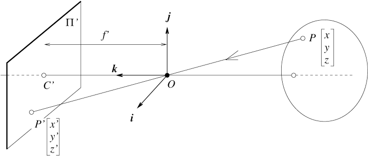
Figure 3: Visualization of the projection equation (Forsyth and Ponce).
Remember that this is not taking optics into account. This is a simple projective model. The figure below shows the relationship between the virtual image plane and sensor image plane.
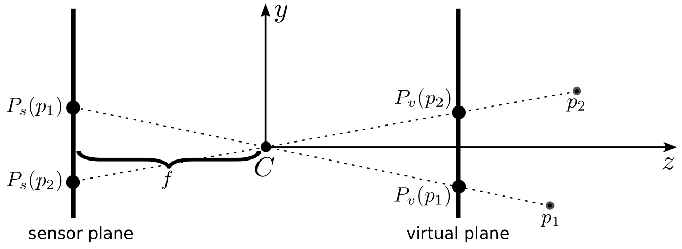
Figure 4: Sensor plane versus virtual plane.
To calculate the points projected to the sensor plane using our simple matrix from above, we only need to negate the \(z\) and \(w\) values:
\[ M = \begin{bmatrix} 1 & 0 & 0 & 0\\ 0 & 1 & 0 & 0\\ 0 & 0 & -1 & 0\\ 0 & 0 & -1 & 0\\ \end{bmatrix} \]
Then the transformed point becomes
\[ M\mathbf{p} = \begin{bmatrix} x\\ y\\ -z\\ -z \end{bmatrix}. \]
Applying the perspective divide yields the 3D point \((-\frac{x}{z}, -\frac{y}{z}, 1)\).
Considering the Focal Length
An important property that all cameras have is the focal length \(f\). That is the distance between the lens and the camera’s sensor. In computer graphics terms, the focal length may also refer to the distance between the virtual image plane and camera. This is then called the near plane instead.
For the following examples, we will follow OpenGL’s projective matrix in which the \(x\) and \(y\) values are scaled by a relationship between the focal length and image window size:
\[ \frac{2n}{r - l}, \]
where \(n\) is the near plane distance (related to \(f\)), \(r\) is the value of the right side of the window, and \(l\) is the value of the left side of the window. For a square window of size \([-1, 1]\), this reduces to \(n\) (or \(f\)). Then the projection matrix is given as
\[ M = \begin{bmatrix} 1 & 0 & 0 & 0\\ 0 & 1 & 0 & 0\\ 0 & 0 & -\frac{1}{f} & 0\\ 0 & 0 & -1 & 0\\ \end{bmatrix}. \]
Why does \(M(3, 3) = -\frac{1}{f}\)?
The projected point should be \(f\) units away from the lens. Projecting a point using the matrix above yields
\[ M\mathbf{p} = \begin{bmatrix} x\\ y\\ -\frac{z}{f}\\ -z \end{bmatrix}. \]
Then applying the perspective divide to compute the projected coordinate results in
\[ \mathbf{p’} = \begin{bmatrix} -\frac{fx}{z}\\ -\frac{fy}{z}\\ \end{bmatrix}. \]
We first computed the 3D homogeneous coordinate and then applied the relationship to 2D homogeneous coordinates using the resulting \((x, y, z)\) triplet. Applying the final divide which establishes the relationship between 2D Cartesian and homogeneous coordinates results in \(\mathbf{p’}\).
Be aware that computer graphics implementations may apply this process differently using a matrix that looks something like this
\[ M = \begin{bmatrix} f & 0 & 0 & 0\\ 0 & f & 0 & 0\\ 0 & 0 & -1 & 0\\ 0 & 0 & -1 & 0\\ \end{bmatrix}. \]
If we apply this to a point in 3D space using homogeneous coordinates, it results in the point
\[ M\mathbf{p} = \begin{bmatrix} fx\\ fy\\ -z\\ -z \end{bmatrix}. \]
Then the resulting 3D point is
\[ \mathbf{p’} = \begin{bmatrix} -\frac{fx}{z}\\ -\frac{fy}{z}\\ 1\\ \end{bmatrix}, \]
which gives us the same \(x\) and \(y\) values of the projected point as before.
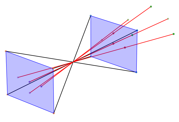
Figure 5: 3D points (green) projected onto the virtual plane (red) and sensor plane (blue).
From World Space to Image Space
The process of projecting points in camera space onto an image plane is fairly simple, but gets slightly more complicated when considering each entity from the world perspective. Objects in the world appear differently depending on the viewpoint of the camera. To model this mathematically, we need to be able to describe the points in 3 different spaces:
- World space
- Camera space
- Image space
To fully describe the possibilities that our camera’s perspective can take, we need to define scaling, translation, and rotations. These allow us to describe the different positions and orientations are camera may be in with respect to the world around it.
Translation
Consider the points of a pyramid observed by a virtual camera, as seen below.
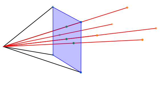
Figure 6: Points of a pyramid as seen from our virtual camera.
If we move the camera away from the points, the will appear smaller (assuming a perspective projection). This movement is described by a translation with respect to the origin in world space. In the above figure, the camera is position at the origin. The figure below shows the camera moved down the $z$-axis by 2 units.
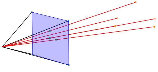
Figure 7: Translating the camera backwards by 2 units. The project points appear smaller.
This is described with a matrix as
\[ T = \begin{bmatrix} 1 & 0 & 0 & -2\\ 0 & 1 & 0 & 0\\ 0 & 0 & 1 & 0\\ 0 & 0 & 0 & 1\\ \end{bmatrix}. \]
In general, a translation in 3D can be described with the following matrix
\[ T = \begin{bmatrix} 1 & 0 & 0 & T_x\\ 0 & 1 & 0 & T_y\\ 0 & 0 & 1 & T_z\\ 0 & 0 & 0 & 1\\ \end{bmatrix}. \]
Scaling
Projected objects can appear larger or smaller depending on the focal length and field of view. Recall the perspective projection matrix from the previous section:
\[ P = \begin{bmatrix} f & 0 & 0 & 0\\ 0 & f & 0 & 0\\ 0 & 0 & -1 & 0\\ 0 & 0 & -1 & 0\\ \end{bmatrix}. \]
The projections we have seen so far are with a focal length of 1. We can make the objects in the image appear larger by increasing the focal length, as seen below.
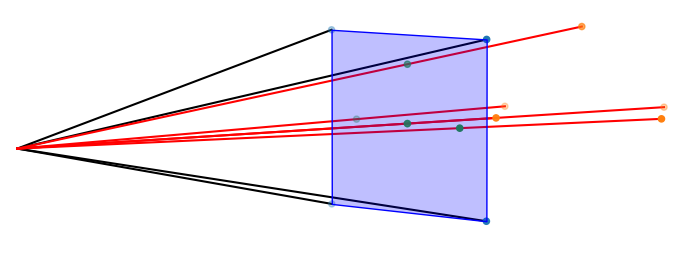
Figure 8: Focal length doubled. The projected image appears larger.
Rotation
Finally, we can rotate our camera about the \(x\), \(y\), or \(z\) axis. Following a right-handed coordinate system, these rotations are given by
\begin{align*} R_x(\theta) &= \begin{bmatrix} 1 & 0 & 0\\ 0 & \cos \theta & -\sin \theta\\ 0 & \sin \theta & \cos \theta \end{bmatrix}\\ R_y(\theta) &= \begin{bmatrix} \cos \theta & 0 & \sin \theta\\ 0 & 1 & 0\\ -\sin \theta & 0 & \cos \theta \end{bmatrix}\\ R_z(\theta) &= \begin{bmatrix} \cos \theta & -\sin \theta & 0\\ \sin \theta & \cos \theta & 0\\ 0 & 0 & 1 \end{bmatrix}\\ \end{align*}
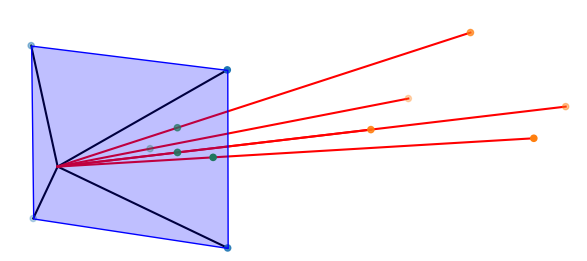
Figure 9: Rotating the camera about the y-axis. The points now appear on the right side of the image plane.
Camera Parameters
When relating points in the world to those of the image space, two sets of parameters are typically used: the intrinsic and extrinsic parameters of a camera. Intrinsic parameters relate the points in the camera’s reference frame to those of the image plane. Extrinsic parameters relate the camera’s coordinate system to a world coordinate system as well as describing its position and orientation.
Intrinsic Parameters
Which parameters are required to project a point to the image plane? The intrinsic parameters are those which convert the points on the physical sensor into a normalized image frame. We start with a basic projection matrix
\[ M = \begin{bmatrix} 1 & 0 & 0 & 0\\ 0 & 1 & 0 & 0\\ 0 & 0 & -1 & 0\\ 0 & 0 & -1 & 0\\ \end{bmatrix}. \]
A physical sensor may not have square pixels, so there are two additional scale parameters \(k\) and \(l\). Along with the focal length \(f\), the projected values become
\begin{align*} x &= kf\frac{X}{Z} = kf\hat{x}\\ y &= lf\frac{Y}{Z} = lf\hat{y}\\ \end{align*}
The focal length and scale factors \(k\) and \(l\) are dependent and can be written as \(\alpha = kf\) and \(\beta = lf\).
The physical sensor has an origin at the corner whereas the normalized image frame has an origin at the center. To account for this offset, a translation parameter for both \(x\) and \(y\) is necessary. The pixel conversion is now represented as
\begin{align*} x &= \alpha \hat{x} + x_0\\ y &= \beta \hat{y} + y_0\\ \end{align*}
Finally, the sensor may not be perfectly center. There may also be additional defects that cause the sensor to be warped or skewed. This is error that can be accounted for by a rotation.
\begin{align*} x &= \alpha \hat{x} - \alpha \cot \theta \hat{y} + x_0\\ y &= \frac{\beta}{\sin \theta} \hat{y} + y_0\\ \end{align*}
To recap, the 5 intrinsic parameters are
- \(\alpha\) - scale parameter for \(x\)
- \(\frac{\beta}{\sin \theta}\) - scale parameter for \(y\), also accounts for skew
- \(-\alpha \cot \theta\) - skew coefficient between the \(x\) and \(y\) axis
- \(x_0\) - the principal point for \(x\)
- \(y_0\) - the principal point for \(y\)
The third parameter \(-\alpha \cot \theta\) is sometimes represented as \(\gamma\) and will be set to 0 in most cases. A typical intrinsic matrix is then
\[ K = \begin{bmatrix} \alpha & \gamma & x_0\\ 0 & \beta & y_0\\ 0 & 0 & 1\\ \end{bmatrix}. \]
Extrinsic Parameters
Given a point with respect to the world frame, \([\mathbf{p}]_W\), we are interested in a change of basis matrix which transforms the world space coordinate to the camera’s basis. This is represented by a change of basis matrix which converts a point in world space to the camera’s coordinate frame.
The matrix is defined as a rigid transformation involving a rotation and translation. The rotation components \(R\) are composed following the 3 rotation matrices described earlier. This only requires 3 parameters if using something like Euler angles. Euler angles represent the rotational angle around each axis by individual parameters \(\phi\), \(\theta\), and \(\psi\).
\[ R = \begin{bmatrix} r_{11} & r_{12} & r_{13}\\ r_{21} & r_{22} & r_{23}\\ r_{31} & r_{32} & r_{33}\\ \end{bmatrix} \]
The translational component is represented using an additional 3 parameters \(t_x\), \(t_y\), and \(t_z\). This can be represented as a matrix
\[ T = \begin{bmatrix} 1 & 0 & 0 & t_x\\ 0 & 1 & 0 & t_y\\ 0 & 0 & 1 & t_z\\ \end{bmatrix}. \]
For convenience, the extrinsic parameters can be represented as a single matrix
\[ M = \begin{bmatrix} r_{11} & r_{12} & r_{13} & t_x\\ r_{21} & r_{22} & r_{23} & t_y\\ r_{31} & r_{32} & r_{33} & t_z\\ \end{bmatrix} \]
The full transformation from world space to image space is then represented as
\[ \mathbf{p} = KM[\mathbf{p}]_W, \]
where \([\mathbf{p}]_W = \begin{bmatrix}x\\y\\z\\1\end{bmatrix}\).
Estimating Camera Parameters
There are many applications which require that we know the exact camera parameters, including augmented reality, inpainting techniques, and depth estimation. We now investigate how, given a fixed world coordinate system with known structure, we can approximate the camera parameters.
Consider a set of \(n\) image-to-world point correspondences \(\mathbf{X}_i \leftrightarrow \mathbf{x}_i\). The goal is to compute a homography \(\mathbf{H}\) that relates the image points to the world points: \(\mathbf{x}_i = \mathbf{H}\mathbf{X}_i\). This relationship can be written as \(\mathbf{x}_i \times \mathbf{H}\mathbf{X}_i = 0\) because the cross product of two vectors is zero if they are parallel. \(H\mathbf{x}_i\) can be written as
\begin{pmatrix} \mathbf{h}_1^T\mathbf{x}_i\\ \mathbf{h}_2^T\mathbf{x}_i\\ \mathbf{h}_3^T\mathbf{x}_i\\ \end{pmatrix}
Then the cross product is given by
\begin{pmatrix} y_i\mathbf{h}_3^T\mathbf{X}_i - w_i\mathbf{h}_2^T\mathbf{X}_i\\ w_i\mathbf{h}_1^T\mathbf{X}_i - x_i\mathbf{h}_3^T\mathbf{X}_i\\ x_i\mathbf{h}_2^T\mathbf{X}_i - y_i\mathbf{h}_1^T\mathbf{X}_i\\ \end{pmatrix}
Observing that \(\mathbf{h}_j^T\mathbf{X}_i = \mathbf{X}_i^T\mathbf{h}_j\), we can write this as a homogeneous linear system.
\[ \begin{bmatrix} \mathbf{0}^T & -w_i\mathbf{X}_i^T & y_i\mathbf{X}_i^T\\ w_i\mathbf{X}_i^T & \mathbf{0}^T & -x_i\mathbf{X}_i^T\\ -y_i\mathbf{X}_i^T & x_i\mathbf{X}_i^T & \mathbf{0}^T\\ \end{bmatrix} \begin{pmatrix} \mathbf{h}_1\\ \mathbf{h}_2\\ \mathbf{h}_3\\ \end{pmatrix} = \mathbf{0} \]
This is a linear system whose third equation is linearly dependent on the first two, thus we only need to solve the first two equations.
\[ \begin{bmatrix} \mathbf{0}^T & -w_i\mathbf{X}_i^T & y_i\mathbf{X}_i^T\\ w_i\mathbf{X}_i^T & \mathbf{0}^T & -x_i\mathbf{X}_i^T\\ \end{bmatrix} \begin{pmatrix} \mathbf{h}_1\\ \mathbf{h}_2\\ \mathbf{h}_3\\ \end{pmatrix} = \mathbf{0} \]
In practice, this system is denoted as \(A_i \mathbf{h} = \mathbf{0}\) where \(A_i\) is a \(2 \times 9\) matrix and \(\mathbf{h}\) is a \(9 \times 1\) vector. This implies that we need at least 4 point correspondences to solve for \(\mathbf{h}\). These correspondences can be used to create 4 matrices \(A_i\) which are then stacked to form a \(8 \times 9\) matrix \(A\). But wait… \(A\) is only rank 8! This is because the solution can only be determined up to a scale factor.
If we the matrix had rank 9, then the solution would be trivial. Remember, we’re working with a homogeneous linear system.
Relationship to Camera Parameters
Given the basic solution, let’s relate this to the camera parameters. Our goal is to estimate \(P\) which is a \(3 \times 4\) matrix. This matrix is composed of the intrinsic matrix \(K\) and the extrinsic matrix \(M\). Since each row of \(P\) is a 4-vector, each \(A_i\) is a \(2 \times 12\) matrix.
Algebraic versus Geometric Error
The solution to the linear system minimizes the algebraic error. Even if the points are perfectly matched, the solution may not be accurate. This is because the solution is only determined up to a scale factor. The geometric error is minimized by using a non-linear optimization technique such as Levenberg-Marquardt.
Application: Camera Calibration
Popular software solutions for calibrating cameras are provided by MATLAB and OpenCV. These are based off of work by Zhengyou Zhang. We will follow the original publication to explain the solutions to camera calibration. As such, the notation will change a bit.
The first goal is to relate the model points \(\mathbf{M}\) to the image points \(\mathbf{m}\) by a homography \(\mathbf{H}\) such that
\[ s\hat{\mathbf{m}} = \mathbf{H} \hat{\mathbf{M}}, \]
where \(\hat{\mathbf{m}}\) is the homogeneous coordinate of \(\mathbf{m}\) (likewise for \(\mathbf{M}\)) and \(s\) is a scale factor.
To relate this to the notation in the previous section,
\[ s\tilde{\mathbf{m}} = \mathbf{H} \tilde{\mathbf{M}} \equiv \mathbf{p} = KM[\mathbf{p}]_W. \]
In the paper, \(\mathbf{H} = \mathbf{A}[\mathbf{R}\quad \mathbf{t}]\), where
\[ \mathbf{A} = \begin{bmatrix} \alpha & \gamma & u_0\\ 0 & \beta & v_0\\ 0 & 0 & 1\\ \end{bmatrix}. \]
\([\mathbf{R}\quad \mathbf{t}]\) is the matrix \(M\) from the previous section.
Estimating the Homography
If we have an image of the model plane, we can estimate \(\mathbf{H}\) using maximum-likelihood estimation as follows. Assume that \(\mathbf{m}_i\) is affected by Gaussian noise with zero mean and covariance \(\mathbf{\Lambda}_{\mathbf{m}_i}\). The objective is then to minimize
\[ \sum_i (\mathbf{m}_i - \hat{\mathbf{m}_i})^T \mathbf{\Lambda_{\mathbf{m}_i}^{-1}}(\mathbf{m}_i - \hat{\mathbf{m}_i}), \]
where
\[ \hat{\mathbf{m}_i} = \frac{1}{\bar{\mathbf{h}}_3^T \mathbf{M}_i} \begin{bmatrix} \bar{\mathbf{h}}_1^T \mathbf{M}_i\\ \bar{\mathbf{h}}_2^T \mathbf{M}_i\\ \end{bmatrix}. \]
\(\bar{\mathbf{h}}_i\) represents the $i$th row of \(\mathbf{H}\).
The approach now constructs a matrix of model points similar to the approach used by RANSAC. First, let \(\mathbf{x} = [\bar{\mathbf{h}}_1^T\ \bar{\mathbf{h}}_2^T\ \bar{\mathbf{h}}_3^T]\). Recalling that \(\widetilde{\mathbf{M}}^T \in [X, Y, 1]^T\),
\[ \begin{bmatrix} \widetilde{\mathbf{M}}^T & \mathbf{0}^T & -u \widetilde{\mathbf{M}}^T\\ \mathbf{0}^T & \widetilde{\mathbf{M}}^T & -v \widetilde{\mathbf{M}}^T\\ \end{bmatrix}\mathbf{x} = \mathbf{0}. \]
Writing this as \(\mathbf{L}\mathbf{x} = \mathbf{0}\), where \(\mathbf{L} \in \mathbb{R}^{2n \times 9}\) with \(n\) being the number of points, the solution the eigenvector of \(\mathbf{L}^T\mathbf{L}\) corresponding to the smallest eigenvalue. This can be computed using Singular Value Decomposition without computing \(\mathbf{L}^T\mathbf{L}\) directly. Factorize \(\mathbf{L} = \mathbf{U}\mathbf{\Sigma}\mathbf{V}^T\) using SVD. Then the parameters that minimizes the objective is the column vector in \(\mathbf{V}\) corresponding to the smallest eigenvalue.
It is noted that since the columns of the rotation matrix are orthonormal, the following constraints are observed:
\begin{align*} \mathbf{h}_1^T \mathbf{A}^{-T} \mathbf{A}^{-1} \mathbf{h}_2 &= 0\\ \mathbf{h}_1^T \mathbf{A}^{-T} \mathbf{A}^{-1} \mathbf{h}_1 &= \mathbf{h}_2^T \mathbf{A}^{-T} \mathbf{A}^{-1} \mathbf{h}_2\\ \end{align*}
Solving for the Camera Parameters
With the homography \(\mathbf{H}\) and constraints given in the last section, Zhang proposes a two step solution that first estimates the parameters using a closed form solution. These serve as a starting point for a non-linear optimization using Levenberg-Marquardt.
First, let
\[ \mathbf{B} = \mathbf{A}^{-T} \mathbf{A}^{-1} = \begin{bmatrix} \frac{1}{\alpha^2} & -\frac{\gamma}{\alpha^2\beta} & \frac{v_0\gamma - u_0\beta}{\alpha^2 \beta}\\ -\frac{\gamma}{\alpha^2\beta} & \frac{\gamma^2}{\alpha^2\beta^2} + \frac{1}{\beta^2} & -\frac{\gamma(v_0\gamma-u_0\beta)}{\alpha^2\beta^2}-\frac{v_0}{\beta^2}\\ \frac{v_0\gamma - u_0\beta}{\alpha^2 \beta} & -\frac{\gamma(v_0\gamma-u_0\beta)}{\alpha^2\beta^2}-\frac{v_0}{\beta^2} & \frac{(v_0\gamma-u_0\beta)^2}{\alpha^2\beta^2}+\frac{v_0^2}{\beta^2}+1 \end{bmatrix}. \]
This is a symmetric matrix which can be represented more compactly as
\[ \mathbf{b} = [B_{11}\ B_{12}\ B_{22}\ B_{13}\ B_{23}\ B_{33}]^T. \]
We can then write \(\mathbf{h}_1^T \mathbf{A}^{-T} \mathbf{A}^{-1} \mathbf{h}_2 = 0\) as
\[ \mathbf{h}_i^T \mathbf{B} \mathbf{h}_j = \mathbf{v}_{ij}^T \mathbf{b}, \]
where
\[ \mathbf{v}_{ij} = [h_{i1}h_{j1}, h_{i1}h_{j2} + h_{i2}h_{j1}, h_{i2}h_{j2}, h_{i3}h_{j1} + h_{i1}h_{j3}, h_{i3}h_{j2}+h_{i2}h_{j3}, h_{i3}h_{j3}]^T. \]
This permits us to write the constraints from the previous section as two homogeneous equations in \(\mathbf{b}\)
\[ \begin{bmatrix} \mathbf{v}_{12}^T\\ (\mathbf{v}_{11} - \mathbf{v}_{22})^T \end{bmatrix} \mathbf{b} = \mathbf{0}. \]
If we compute the homography, as above, on \(n\) images, we end up with \(n\) equations like the one directly above. Stacking this yields
\[ \mathbf{V}\mathbf{b} = \mathbf{0}, \]
where \(\mathbf{V} \in \mathbb{R}^{2n \times 6}\).
The initial set of parameters is then solved following the solution for each homography \(\mathbf{H}\). With \(\mathbf{b}\) estimated, the intrinsic parameters are
\begin{align*} v_0 &= (B_{12}B_{13} - B_{11}B_{23})/(B_{11}B_{22} - B_{12}^2)\\ \lambda &= B_{33} - [B_{13}^2 + v_0(B_{12}B_{13} - B_{11}B_{23})]/B_{11}\\ \alpha &= \sqrt{\lambda / B_{11}}\\ \beta &= \sqrt{\lambda B_{11}/(B_{11}B_{22} - B_{12}^2)}\\ \gamma &= -B_{12}\alpha^2\beta / \lambda\\ u_0 &= \gamma v_0 / \alpha - B_{13} \alpha^2 / \lambda. \end{align*}
The parameters \(\alpha, \beta, \gamma, u_0, v_0\) make up our intrinsic parameter matrix \(\mathbf{A}\). These can be used to compute the extrinsic parameters following
\begin{align*} \lambda &= 1 / \|\mathbf{A}^{-1}\mathbf{h}_1\|\\ \mathbf{r}_1 &= \lambda \mathbf{A}^{-1}\mathbf{h}_1\\ \mathbf{r}_2 &= \lambda \mathbf{A}^{-1}\mathbf{h}_2\\ \mathbf{r}_3 &= \mathbf{r}_1 \times \mathbf{r}_2\\ \mathbf{t} &= \lambda \mathbf{A}^{-1}\mathbf{h}_3\\ \end{align*}
Refining the Estimates
The approach in the last section is produced by minimizing algebraic distances. These values are further refined using maximum-likelihood estimation by way of a nonlinear optimizer. If there are \(m\) points on each of the \(n\) images, the objective function to minimize is given by
\[ \sum_{i=1}^n \sum_{j=1}^m \|\mathbf{m}_{ij} - \hat{\mathbf{m}}(\mathbf{A}, \mathbf{R}_i, \mathbf{t}_i, \mathbf{M}_j)\|^2, \]
where \(\hat{\mathbf{m}}(\mathbf{A}, \mathbf{R}_i, \mathbf{t}_i, \mathbf{M}_j)\) is a projection of point \(\mathbf{M}_j\) in image \(i\). This function is minimized using the Levenberg-Marquardt algorithm.