Convolutional Neural Networks
Key Concepts
- Invariance and Equivariance
- Definition
- Padding, Stride, Kernel size, dilation
- Purpose of multiple feature maps
- Receptive fields and hierarchies of features
- Downsampling, Upsampling, Examples in research
Introduction
Dense neural networks made up of linear layers and a chosen activation function are not practical for image data. Consider an image of size \(224\times224\times3\). The first layer of a dense network would require a \(150,528\times n\) parameter matrix, where \(n\) is the number of nodes in the first layer. It is common to build dense networks where the first layer has more nodes than input features. In this case, we would need a minimum of \(150,528^2\) parameters in the first layer. Even if we chose something much smaller like \(n=1024\), this would require \(154,140,672\) parameters for just the first layer. This is clearly impractical.
Aside from requiring a large number of parameters, we might ask whether it is beneficial to feed raw pixel values into a dense network. The network itself would be learning pixel-wise features with no regard to their spatial relationship. This makes our network’s job much more difficult because the spatial arrangement of features tells us so much about what we see. In practice, this means that the network would have to learn the same features at every location in the image. We would instead prefer this network to learn features that are invariant to translation. That is, the network should learn features that are the same regardless of where they appear in the image.
Invariance to translation is very convenient and can save our network a lot of work in learning the same feature at every point in the input. It is also desirable that our network is invariant to other transformations such as rotation, scaling, skewing, and warping. Formally, a function \(f(\mathbf{x})\) of an image \(\mathbf{x}\) is invariant to a transformation \(t(\mathbf{x})\) if
\[ f(t(\mathbf{x})) = f(\mathbf{x}). \]
Aside from invariance, some models should be equivariant to certain transformations. That is, the output of the model should change in the same way as the input. Image segmentation models should be equivariant to translation. If we were to shift an image by a few pixels, the output segmentation mask should also shift by the same amount. Convolutional neural networks are equivariant to translation.
Convolution Operator
A convolution is a function that takes two functions as input and produces a third function as output. The first function is the input and the second function is the kernel. The output is called the feature map. The kernel is also sometimes called the filter.
\[ (f * g)(t) = \int f(t-a)g(a)da \]
We can view them more concretely by considering the functions to be vectors. For example, let the function \(f\) be an input vector \(x\) and \(w\) be a kernel representing a filter. The convolution operator is then
\[ (x * w)(t) = \int x(t-a)w(a)da. \]
The result the feature map representing the response of the kernel at each location in the input.
In the case of discrete values, the operator is written as
\[ (x * w)(t) = \sum_{a}x(t-a)w(a). \]
In machine learning, the kernel \(w\) is usually represented by some set of parameters that is optimized.
CNNs for images use a 2D convolution defined as
\[ (I * K)(i, j) = \sum_m \sum_n I(i-m, j-n)K(m, n). \]
In this formulation, the kernel is effectively flipped across the vertical and horizontal axis.
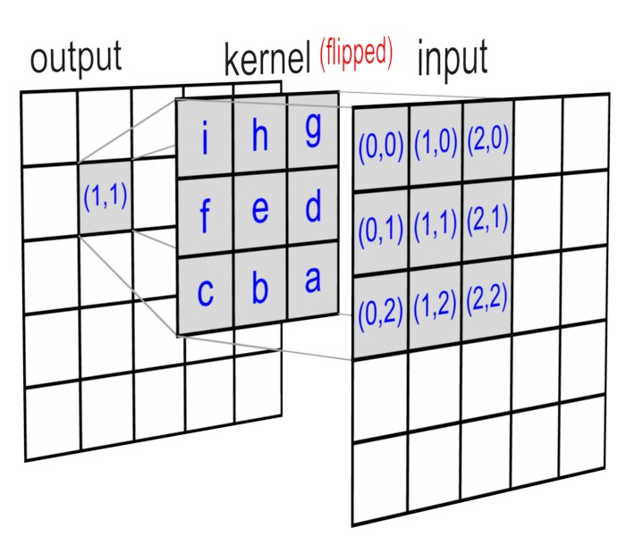
Figure 1: 2D Convolution (Image Credit: Song Ho Ahn (linked above)).
In practice, most deep learning APIs implement cross-correlation. Whether the function is implemented as true convolution makes no difference when it comes to optimizing a deep model since filter weights that are produced with cross-correlation would be produced, albeit flipped, with convolution.
\[ (K * I)(i, j) = \sum_m \sum_n I(i+m, j+n)K(m, n). \]
Properties of Convolutions
Convolutional networks are commonly built on full or valid convolutions. Other variants have also been explored. Here, we will briefly discuss the different properties of this operator. A more detailed treatment can be found in (Dumoulin and Visin 2018).
Padding
By definition, a convolution of an input with a filter of size \(n\times n\) will produce an output of size \((m-n+1)\times(m-n+1)\), where \(m\) is the size of the input. This means that the output will be smaller than the input. This is often referred to as a valid convolution. The figure below shows a convolution between a \(3\times3\) kernel and a \(5\times5\) input.
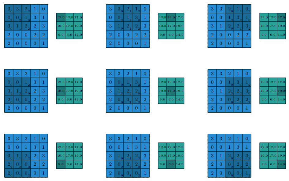
Figure 2: A valid convolution (Dumoulin and Visin 2018).
The output of this convolution is a \(3\times3\) feature map. This is a problem if we want to build a deep network. Each convolution will reduce the size of the input. If we were to stack multiple convolutional layers, the output would eventually be too small to be useful. If we want our output to be same size as the input, we can add padding to the original input image before convolving it. This is often known as a full convolution. An example is shown below.
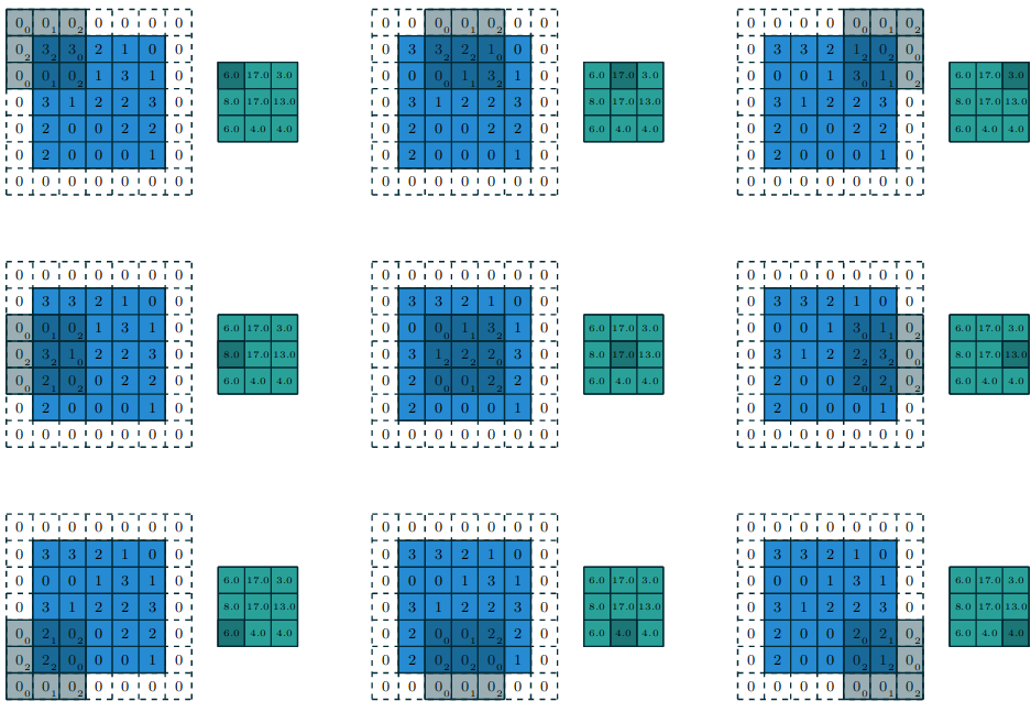
Figure 3: A full convolution (Dumoulin and Visin 2018).
Stride
So far, we have only looked at convolutions which step by 1 unit as they shift over the image. We can control the size of this step, or stride, to produce different outcomes. Picking a non-unit stride has a number of effects on the features that are learned in a convolutional neural network.
- Dimensionality reduction: Skipping over pixels reduces the size of the output feature map. This provides another way of downsampling the input.
- Less computation: Fewer computations are required to produce the output feature map.
- Increased field of view: A larger stride increases the field of view of the kernel, leading to larger receptive fields in deeper layers.
Given an input of size \(m\times m\) and a kernel of size \(n\times n\), the output size of a convolution with stride \(s\) is given by
\[ \left\lfloor\frac{m-n}{s}\right\rfloor + 1. \]
The figure below shows a convolution with stride 2 on a \(5\times5\) input.
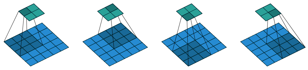
Figure 4: A convolution with stride 2 (Dumoulin and Visin 2018).
Kernel Size
The size of the kernel has a large impact on the features that are learned. A larger kernel will have a larger receptive field. This means that the kernel will be able to capture more information about the input. However, this comes at the cost of increased computation. Common kernel sizes in most CNNs are \(3\times3\), \(5\times5\), and \(7\times7\). It is also convenient to pick an odd kernel size so that the kernel has a center pixel.
Dilation
Around 2015, a research trend for CNNs was to find a way to increase the receptive field without adding more parameters. The result is a dilated convolution. The output of a dilated convolution is computed by skipping over pixels in the input. The figure below shows a \(3\times3\) kernel with a dilation of 2.
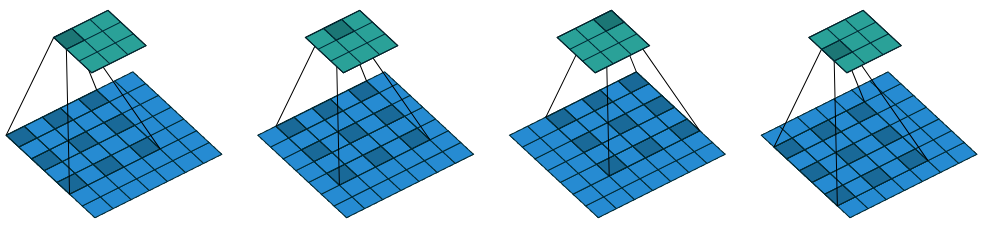
Figure 5: A dilated convolution (Dumoulin and Visin 2018).
The output size is computed as
\[ \left\lfloor\frac{m + 2p - n - (n-1)(d-1)}{s}\right\rfloor + 1, \]
where \(p\) is the amount of padding and \(d\) is the dilation factor.
Parameter Sharing
In a densely connected layer, each input has a corresponding weight attached to it. For example, we ran a few introductory experiments on the CIFAR10 dataset using a deep, densely connected network. To reduce the amount of parameters in the first layer, we converted each image to grayscale. The input also had to be vectorized in order to be processed. With a processed image of size \(32 \times 32\), this resulted in a \(1024\) dimensional vector for each input. Our first layer had \(512\) nodes resulting in a parameter matrix of size \(1024 \times 512\).
Convolution layers have shared parameters, meaning the same parameters are used for each region on the input. A single channel 2D filter of size \(n \times n\) only requires \(n \times n\) parameters. Each kernel is applied to every location in the original input using the same parameters.
Kernels are equivariant to translation because of their shared parameters. That is, as the input changes, the output will change in the same way. Formally, two functions \(f\) and \(g\) are equivarient if
\[ f(g(x)) = g(f(x)). \]
In the context of image features, a kernel applied across an image will produce strong responses in regions that exhibit the same local features. For example, a kernel that detects horizontal lines will produce strong responses across all parts of the image that show a large contrast between vertical pixels.
Pooling
When a convolution is applied to some input image, the resulting output feature map represents the responses of the kernel applied to each location in the image. If this original image were to be shifted by a few pixels, the reponses would also be shifted. In order to increase the robustness of a model to small perturbations such as translation, a pooling layer was historically employed after each non-linear activation following a convolutional layer.
They effectively provide a summary statistic of a local region by selecting the average or maximum responses in a small window. This provides translation invariance since the maximum response will be the same for a region even if it is translated by a small amount. It also acts as a quick way to downsample the image, leading to fewer parameters in the model.
Modern works do not employ pooling operations as often. For example (He et al. 2016) perform dimensionality reduction with \(1 \times 1\) convolutions. (Springenberg et al. 2015) argue that fully convolutional networks can achieve the same performance without max pooling.
“The pooling operation used in convolutional neural networks is a big mistake and the fact that it works so well is a disaster.” - Geoffrey Hinton
Backwards Pass
The parameters of a convolutional layer are updated via backpropagation like any other layer with trainable parameters. Given a kernel \(w\), it is necessary to compute \(\frac{\partial \mathcal{L}}{\partial w_{m’,n’}}\), where \(w_{m’, n’}\) is the \((m’, n’)th\) entry of the kernel. This entry affects all entries in the feature map, so \(\frac{\partial \mathcal{L}}{\partial w_{m’,n’}}\) will sum over all such entries.
To show the gradient calculation, we will assume a convolutional layer with zero padding and unit stride with a square \(2 \times 2\) kernel applied to a square \(3 \times 3\) input. The output map is then \((3 - 2 + 1) \times (3 - 2 + 1) = 2 \times 2\).
\[ \frac{\partial \mathcal{L}}{\partial w_{m’,n’}} = \sum_{i=0}^2 \sum_{j=0}^2 \frac{\partial \mathcal{L}}{\partial x_{i, j}} \frac{\partial x_{i,j}}{\partial w_{m’, n’}} \]
If \(\mathbf{z}^{(l-1)}\) is the output from the previous layer, then
\begin{align*} \frac{\partial x_{i, j}}{\partial w_{m’, n’}} &= \frac{\partial}{\partial w_{m’, n’}} \sum_{m} \sum_{n} w_{m, n} z_{i+m, j+n}^{(l-1)} + b\\ &= \frac{\partial}{\partial w_{m’, n’}} w_{m’, n’}z_{i+m’, j+n’}^{(l-1)}\\ &= z_{i+m’, j+n’}^{(l-1)} \end{align*}
Then \(\frac{\partial \mathcal{L}}{\partial w_{m’,n’}}\) becomes
\begin{align*} \frac{\partial \mathcal{L}}{\partial w_{m’,n’}} &= \sum_{i=0}^2 \sum_{j=0}^2 \frac{\partial \mathcal{L}}{\partial x_{i, j}} z_{i+m’, j+n’}^{(l-1)}\\ &= \frac{\partial \mathcal{L}}{\partial x_{i, j}} * z_{m’, n’}^{(l-1)}. \end{align*}
\(\frac{\partial \mathcal{L}}{\partial x_{i, j}}\) represent the gradients with respect to the feature maps. To match the flipped kernel used in the forward pass, they are flipped in an opposite manner.
Example
Let’s train and evaluate a convolutional neural network on the OG network: LeNet5 (LeCun et al. 1989).
Neural Networks for Image Classification
ILSVRC
The ImageNet Large Scale Visual Recognition Challenge (ILSVRC) is the most popular image classification and object detection challenge starting in 2010. It now exists as the ILSVRC 2012-2017 challenge on Kaggle.
AlexNet
https://code.google.com/archive/p/cuda-convnet/
The network that arguably popuarlized deep learning by achieving a 37.5% top-1 and 17% top-5 error rate on the ILSVRC-2010 test set. This model performed significantly better than leading competitors (Krizhevsky, Sutskever, and Hinton 2017).
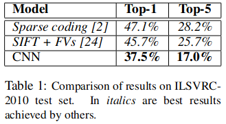
Figure 6: ILSVRC-2010 results reported by Krizhevsky et al.
This performance was based on many different insights and techniques including ReLU activations and dropout. The authors stated in their original publication that the large capacity of the model is necessary to fully describe the diversity of objects in ImageNet.
Architecture
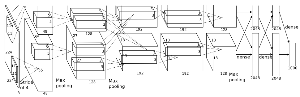
Figure 7: AlexNet architecture (from Krizhevsky et al.)
AlexNet is made up of 5 convolutional layers followed by 3 fully-connected layers. The outputs of the last layer are used as input to the softmax function.
Each layer uses the ReLU activation function.
\[ f(x) = \max(0, x) \]
The justification for switching to ReLU as opposed to sigmoid or tanh is the faster training times. Experiments on smaller CNNs show that networks with ReLU reach 25% training error on CIFAR-10 six times faster than those with tanh activations.
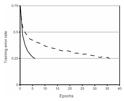
Figure 8: Training loss over time using ReLU (solid) versus tanh (dotted) (from Krizhevsky et al.)
Another benefit of ReLU activations is that they are less reliant on input normalization. In a saturating activation function like tanh, large absolute values in the inputs will be clamped to either -1 or 1. ReLU is unbounded above 0. Networks can still train as long as some input is positive. Local response normalization (LRN) is used after the first and second convolutional layers.
The motivation behind LRN is taken from lateral inhibition in neurobiology. An overly excited neuron (one with a high response) can subdue or dampen the responses from local neighbors. If all responses in a local region are uniformly large, which can happend since ReLU is unbounded, it will dampen them all.
In practice, they showed that applying LRNs to their model reduced the top-1 and top-5 error rates by 1.4% and 1.2%, respectively.
Regularization
The entire network has 60 million parameters. Even with so many parameters and training on a dataset with over 8 million images, their model overfits the training data quickly without the aid of regularization. They employ both image translations and horizontal reflections.
The use of translations is where the popular \(224 \times 224\) training size originated. The original size of the images in the dataset is \(256 \times 256\). To work with random translations without worrying about padding, they crop the final output to \(224 \times 224\). The final output of the network extracts 5 \(224 \times 224\) patches from the test input and averages the network prediction made on each patch.
Additionally, they alter the RGB intensities so that the network is less reliant on specific intensities and illumination for each object. The intuition is that the identity of an object is invariant to lighting conditions.
As a last form of regularization, they employ dropout in the first two fully-connected layers.
Training
They trained their model on a training set of 1.2 million images using two NVIDIA GTX 580 3GB GPUs. They had to write their own optimized CUDA code for this since deep learning frameworks such as Tensorflow and PyTorch did not exist yet. The training took ~6 days to pass 90 epochs.
VGG
Published in 2015, (Simonyan and Zisserman 2015) explore how depth plays a role in convolutional neural networks. They systematically increase the depth of the network while keep other hyperparameters fixed. The filter sizes are also kept at \(3 \times 3\).
Similar to (Krizhevsky, Sutskever, and Hinton 2017), they use ReLU activations and in only one of their models to they employ Local Response Normalization. They found that adding LRN to their model did not increase performance. Instead, it only increased computation time and memory consumption. Their models are summarized in the table below.
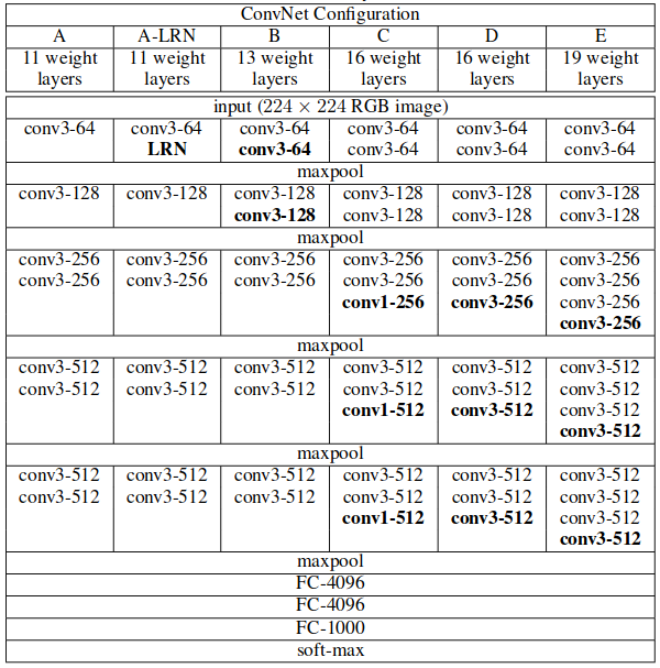
Figure 9: Model configurations used (Simonyan and Zisserman).
The number of parameters for each network is 133 million, 133 million, 134 million, 138 million, and 144 million starting from A to E.
GoogLeNet
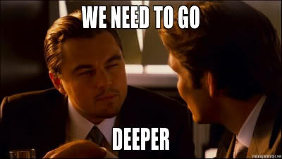
Figure 10: The network-in-network architecture pairs perfectly with the Inception meme.
Proposed a 22-layer network architecture that has \(12 \times\) fewer parameters than (Krizhevsky, Sutskever, and Hinton 2017).
The authors were already thinking about applications in mobile computing, where hardware limitations would require smaller networks that still perform well.
“In this paper, we will focus on an efficient deep neural network architecture for computer vision, codenamed Inception, which derives its name from the Network in network paper by Lin et al. in conjunction with the famous “we need to go deeper” internet meme.” - Szegedy et al.
It was apparent at the time that building larger networks would generally lead to better performance. Adding more parameters leads to easier overfitting. Bigger networks also mean more computation. If the goal is to adapt high quality networks into mobile computing, solutions would have to include more sophistication than simply adding more components.
Hebbian Learning
A linear increase in filters leads to a quadratic increase in computation. If most filter parameters end up being close to 0, then this increase in model capacity is wasted. One solution is to include sparsity in the network instead of having dense connections. Szegedy et al. were motivated by the work of Arora et al., which they summarized as follows.
“Their main result states that if the probability distribution of the data-set is representable by a large, very sparse deep neural network, then the optimal network topology can be constructed layer by layer by analyzing the correlation statistics of the activations of the last layer and clustering neurons with highly correlated outputs.” - Szegedy et al.
This result relates with Hebbian theory on synaptic plasticity which is summarized as “neurons that fire together, wire together.”
From Theory to Architecture
Motivated by sparse connections, the architecture is designed to approximate sparsity given current dense components like convolutional layers.
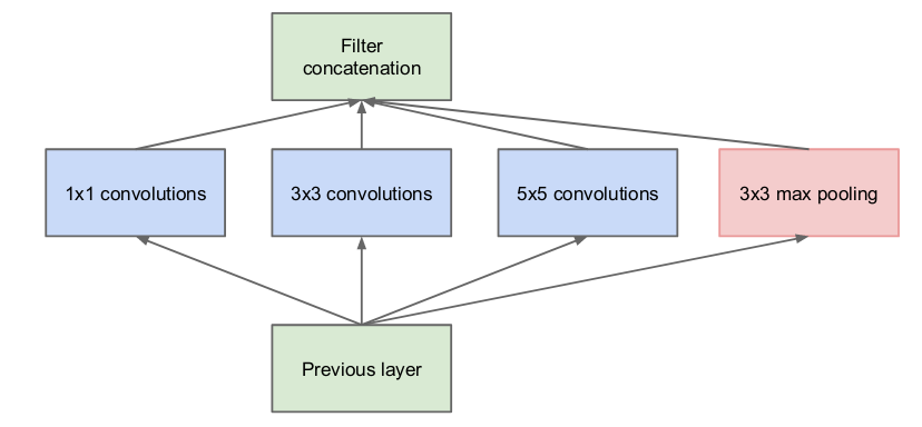
Figure 11: Naive version of the Inception module (Szegedy et al.)
The Inception module design as seen above is motivated as follows. In layers closer to the raw input, filters would be grouped into local regions. In this case, a \(1 \times 1\) convolution would summarize these groups.
For clusters that are spread out, a larger filter would be needed to cover the larger regions. This motivates the use of \(3 \times 3\) and \(5 \times 5\) filters.
The choice to include a max pooling function in each module is based on previous successes of using max pooling.
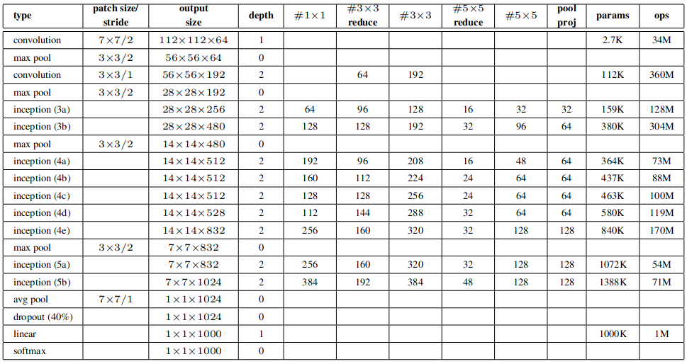
Figure 12: Description of layers from Szegedy et al.
Vanishing Gradients
Creating a deeper network means that training is more susceptible to the vanishing gradient problem. They noted that shallower networks that perform well on image classification would surely provide strong disciminative features. They leverage this idea by computing 2 additional intermediate outputs: one in the middle of the network and an additional output 3 layers beyond that one. This permits the gradients to be strengthened by intermediate losses when combined with the original gradients.
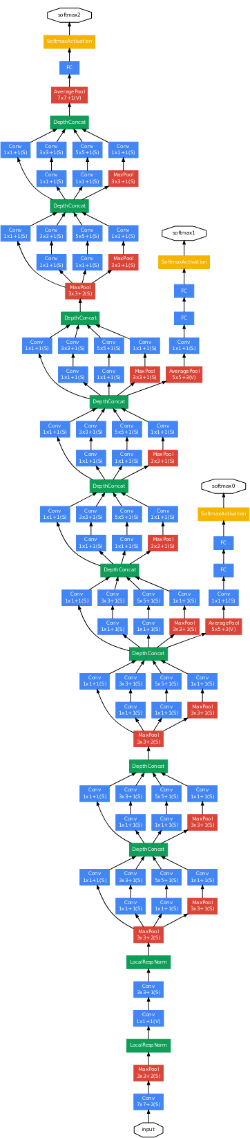
Figure 13: GoogLeNet model (Szegedy et al.)
Results
GoogLeNet took 1st place in the 2014 ILSVRC with a 6.67% top-5 error rate.
ResNet
By 2016, it was clear that deeper models could build a richer hierarchy of features leading to better performance on a wide range of computer vision tasks. However, with deeper networks comes the vanishing gradient problem. Training them remained difficult for a time, but initialization and other normalization techniques found ways to resolve this issue.
With deeper networks, a new problem appeared. Adding more layers generally results in higher accuracy. At a certain point, adding additional layers leads to a decrease in accuracy. Many experiments ruled out the possibility of overfitting by observing that the training error was increasing as well.
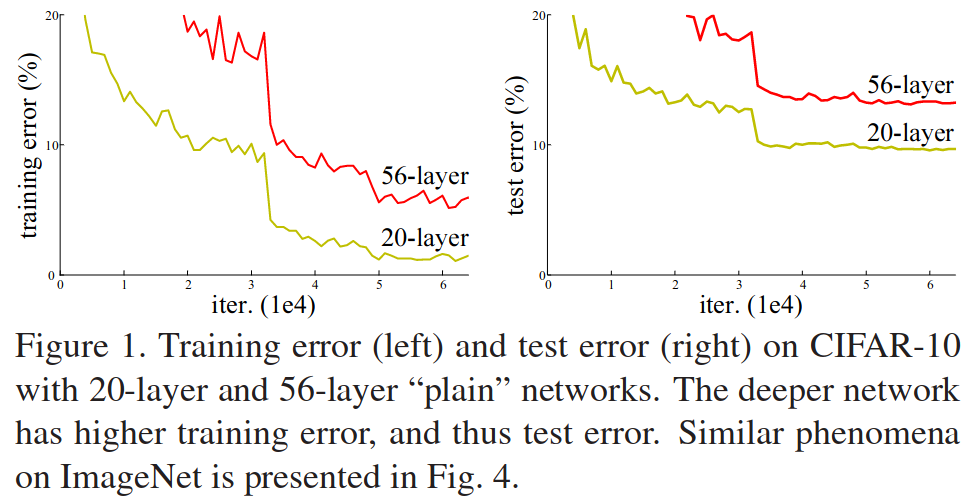
Figure 14: Result of experiments showing that decreased accuracy was not a result of overfitting.
Identity Mappings
Consider a shallow network with some measure performance on a task. If we were to add additional layers to make this network deeper, but those layers were simply identity mappings, then we should expect an error no greater than the original shallow network. However, current solvers are unable to find such a solution in a reasonable amount of time on an equally deep network optimized from a random initialization.
Residual Functions
The main idea of this paper is to attempt to learn a residual function \(\mathcal{F}(\mathbf{x}) := \mathcal{H}(\mathbf{x}) - \mathbf{x}\) of the desired mapping \(\mathcal{H}(\mathbf{x})\) rather than attempting to learn the mapping directly. The desired mapping then given by \(\mathcal{H}(\mathbf{x}) = \mathcal{F}(\mathbf{x}) + \mathbf{x}\). If it were optimal to learn an identity mapping, the idea is that it would be simpler to learn by moving towards a 0 residual.
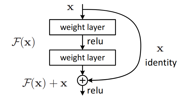
Figure 15: Residual unit (He et al.)
The function can be implemented into neural networks by using skip connections, as seen in the figure above. Adding these identity mappings does not require any additional parameters, as the input is simply passed to the end of the stack.
Architecture Complexity
They compare a 34-layer plain network based on the VGG-19 architecture with a 34-layer residual network. They note that VGG-19 has more filters and higher complexity than their residual network. Specifically, VGG-19 requires 19.6 billion FLOPs compared to only 3.6 billion for their 34-layer residual network.
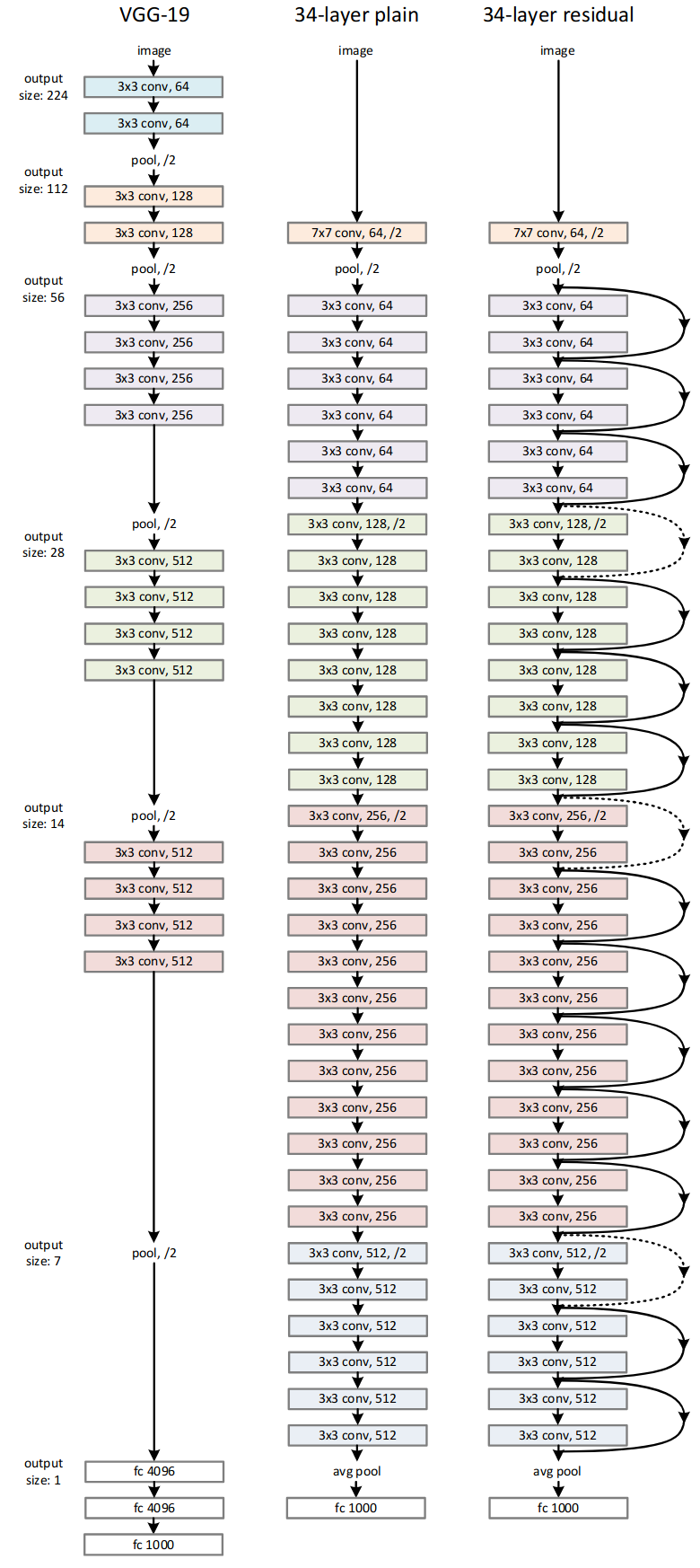
Figure 16: Comparison of architectures and their complexity (He et al.)
Results
They evaluate how well the residual networks generalize when adding more layers. As mentioned in the introduction, typical models would see an increase in training error as the number of layers were increased.
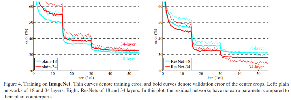
Figure 17: Training comparisons between plain and residual networks (He et al.)
Their ensemble of models achieved 3.57% top-5 error on the ImageNet test set, achieving 1st place in the ILSVRC 2015 classification challenge. It additionally was adapted to other challenges and won first place on ImageNet detection, ImageNet localization, COCO detection, and COCO segmentation in both the ILSVRC and COCO 2015 competitions.
Useful Resources
- https://www.songho.ca/dsp/convolution/convolution.html#convolution_2d
- https://github.com/vdumoulin/conv_arithmetic
- https://cs231n.github.io/convolutional-networks/
- https://www.jefkine.com/general/2016/09/05/backpropagation-in-convolutional-neural-networks/
- https://grzegorzgwardys.wordpress.com/2016/04/22/8/