CUDA Memory Architecture
The slides accompanying these lecture notes can be found here.
Introduction
So far, the kernels we have used assume everything is on global memory. Even though there are thousands of cores that can effectively hide the latency of transferring data to and from global memory, we will see this delay will become a bottleneck in many applications. These notes explore the different types of memory available on the GPU and how to use them effectively.
Memory Access
Transferring memory is one of the biggest bottlenecks in GPU programming. Companies like NVIDIA devote a lot of resources to improving the bandwidth and latency of memory transfers. When training a deep learning model, the datasets used are far too large to fit on the GPU. This means that the data must be transferred to the GPU before the actual training code can execute on the device. Training large models can take days or weeks, so the time spent transferring data can be significant.
The example provided in Chapter 5 of “Programming Massively Parallel Processors” is a great introduction to understanding memory access efficiency (Hwu, Kirk, and El Hajj 2022). In matrix multiplication, the data accesses are limited to a single line of code in the inner-most loop. This means that the memory access pattern is very regular and predictable. The example code is shown below:
for (int k = 0; i k < numCols; k++) {
    Cvalue += A[row * numCols + k] * B[k * numCols + col];
}
This line consists of a floating-point multiplication, floating-point addition, and two memory accesses. Note that we are not storing the result yet, so there is no access to the C matrix. The operation effiency can be described in terms of floating-point operations per second (FLOP/s) and the accesses can be measured in the number of bytes transferred. In this case, we have 2 FLOPs and 8 bytes transferred. This means that the ratio of FLOPs to bytes transferred is 0.25 FLOP/B. This is described as computational intensity.
With this definition, we get a clearer picture on how to improve the performance of our code. If our kernel relies on too many memory accesses, then the computational intensity will be low. This means that the GPU will be spending more time waiting for data to be transferred than actually performing computations. The goal is to increase the computational intensity as much as possible.
To put this in perspective, the H100 SXM5 has 3TB/s of memory bandwidth. This global memory bandwidth limits the kernel to 3000 * 0.25 = 750 GFLOP/s. The peak performance of the H100 is 66.9 TFLOPS. If the specialized Tensor cores are utilized, the peak performance is 494.7 TFLOPS. That means that our kernel is only using 0.15% of the peak performance of the GPU. This program is certainly memory bound. Our theoretical limit to computational intensity is the peak performance of the GPU. Programs that achieve this peak are called compute bound.
Based on the tools we have discussed so far, it is not clear how we can optimize this kernel. The only way to improve the computational intensity is to reduce the number of memory accesses. Modern GPUs have more than just global memory. The next section will explore the different types of memory available on the GPU.
Memory Types
- Global Memory
- Local Memory Resides on global memory, but is not shared between threads. This includes local variables and function arguments.
- Shared Memory Resides on the chip. Allocated to thread blocks. Shared between threads in the same block.
- Constant Memory
- Registers Resides on the chip. Each thread has its own registers. Very fast memory.
Data in CPU registers are swapped depending on the context of the program. GPU registers are consistent even when other threads are launched to hide latency. This results in a larger register file on the GPU.
Following the von Neumann architecture, memory that is closer to the chip is faster but more expensive. Data residing on registers is the most ideal for performance since the processor can work directly with the register values. This benefit comes in the form of energy consumption as well. Transferring data from global memory to the chip requires additional cycles resulting in more energy used.
When a private variable is declared in a kernel, every single thread will have its own copy of that variable.
| Variable declaration | Memory | Scope | Lifetime |
|---|---|---|---|
| Automatic variables (not arrays) | Register | Thread | Grid |
| Automatic array variables | Local | Thread | Grid |
__device__ __shared__ int SharedVar; |
Shared | Block | Grid |
__device__ int GlobalVar; |
Global | Grid | Application |
__device__ __constant__ int ConstVar; |
Constant | Grid | Application |
Automatic array variables should seldom be used. It may have seemed convenient to use a static array for computing channel-specific values in an image processing kernel, but it is more efficient to use three separate variables. Each variable will be allocated to a register resulting in faster access times.
Global variables are more commonly used to pass information to another kernel that is being launched.
Tiling
These memory types serve as tools that we can use to increase efficiency. The first pattern discussed is tiling. Throughout the rest of the course, we will add many more patterns to our repertoire. Tiling is a well-described technique that has a fitting analogy. If a wall needs to be tiled, it is more efficient to use many small tiles that are lighter and easier to handle. In GPU programming, the wall represents the entire global memory space. The individual tiles are local memory that is allocated to each thread block.
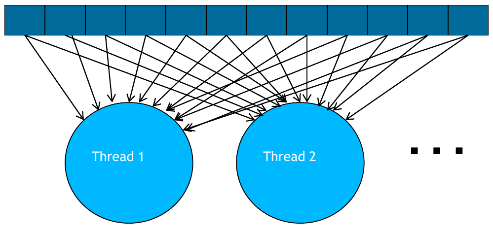
Figure 1: Global memory access pattern (source: NVIDIA DLI).
The kernels we have seen so far have used a global memory access pattern. In this pattern, all threads have access to every data point from the input. Using a tiling pattern, we can optimize memory accesses by moving shared resources to local memory that is faster to access.
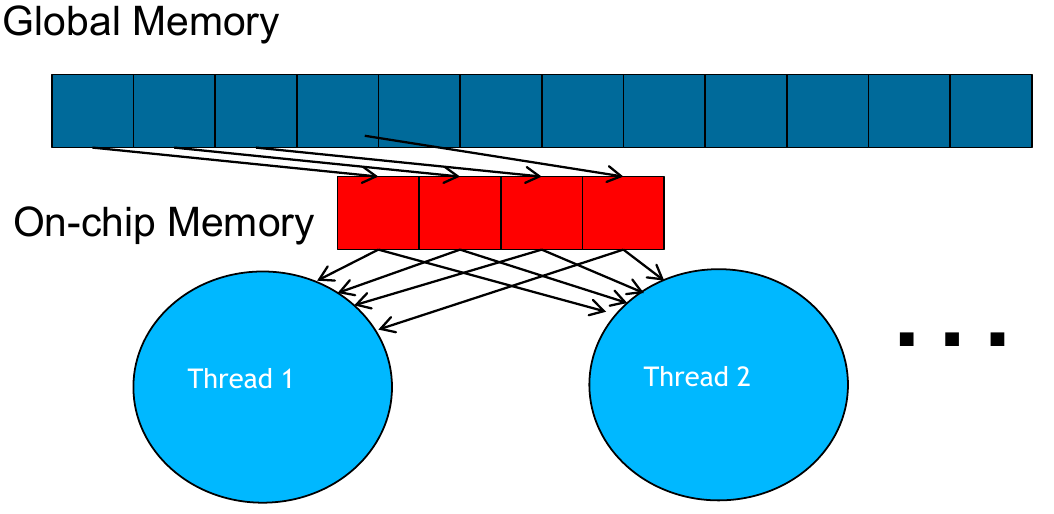
Figure 2: Tiling pattern (source: NVIDIA DLI).
The tool itself is quite simple in concept, but the challenge will be identifying when the tool can be properly applied. Consider matrix multiplication. The naive kernel we explored previously uses each thread to compute one value of the output matrix. This kernel uses a global memory access pattern, and we can identify that many of the computations require the same input. They key to introducing tiling for matrix multiplication will be identifying which data are reused.
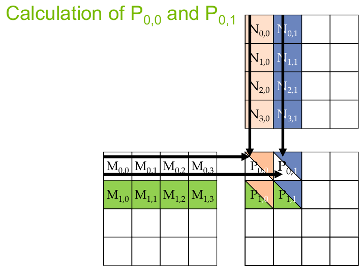
Figure 3: Memory accesses for matrix multiplication (source: NVIDIA DLI).
In the figure above, the block size is \(2 \times 2\). Each row of the block relies on the same input row from the matrix on the left. That is, \(P_{0,0}\) and \(P_{0,1}\) will use the same data from the first row of \(M\). In our original kernel, this requires 8 global memory accesses. If we placed this row in shared memory, each output thread could access the values much quicker. We can see a similar pattern for the column values in \(N\).
Since we are using tiling with a block size of \(B\), we will consider working with \(2B\) values from the input at a time. If the number of values we need to compute an output entry exceeds \(2B\), then we can synchronize the threads before moving to the next section.
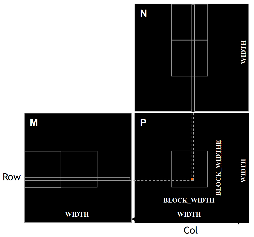
Figure 4: Tiled matrix multiplication overview (source: NVIDIA DLI).
- Verify that the potential reduction in global memory traffic in matrix multiplication is proportional to the dimension of the blocks used.
- Verify that the reduction is by a factor of \(N\) if the tiles are \(N \times N\).
Example: Tiled Matrix Multiplication
The concept of tiled matrix multiplication is this: load a subset of data from \(M\) and \(N\) into shared memory before using that data to perform the dot product. We have a few limitations to think about here. First, the amount of shared memory is much smaller than global memory; we cannot fit all the data at once. Second, the block size will limit how many elements can be loaded into shared memory at once. As suggested by tiling, we are only working with a small chunk at a time.
Using a \(2 \times 2\) block gives us 4 threads to work with. Overlaying that block on the input only allows us to grab 2 values from the first 2 rows in \(M\) and 2 values from the first 2 columns in \(M\). For each tile, the subset of data will be loaded in followed by adding the dot product of the subset to the current value.
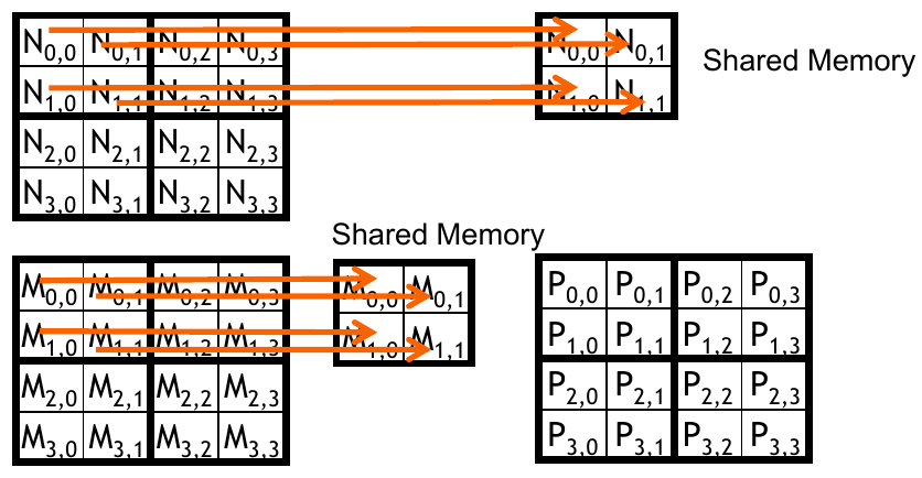
Figure 5: Loading the first tile (source: NVIDIA DLI).
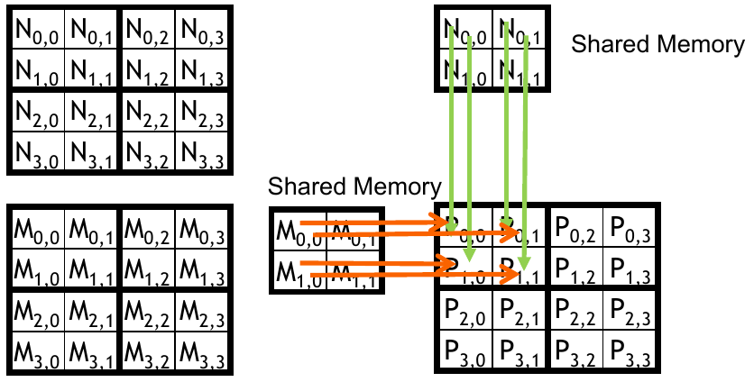
Figure 6: Computing the dot product of the first subset (source: NVIDIA DLI).
In this example, the block will move to the next subset of data to finish computing the first block of the output matrix. This process can be arbitrarily scaled up to support larger matrices without necessarily increasing the block size. Although, we would want to increase the block size to take advantage of the additional threads. The figure below shows a table of the computations required for each phase.
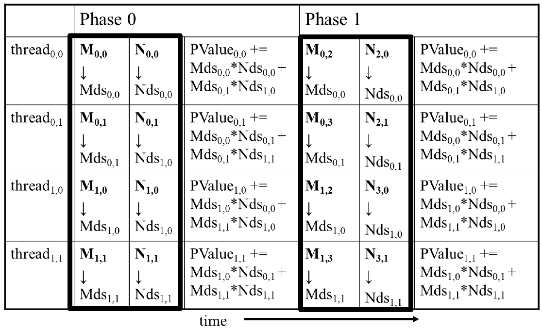
Figure 7: Tiled matrix multiplication computations (source: NVIDIA DLI).
Check your understanding
By using tiling with a block size of \(B \times B\), what is the total reduction in global memory traffic?
Implementation in CUDA
Our implementation should follow these steps:
- Establish shared memory for the input from matrix \(M\) and matrix \(N\).
- Load the first subset of data from \(M\) and \(N\) into shared memory (remember to synchronize threads).
- Compute the dot product of the subset (remember to synchronize threads).
- Repeat steps 2 and 3 until all subsets have been computed.
Step 1 is obvious. We need to establish the shared memory for this solution. Steps 2 and 3 are the same as described above, but we do need to remember to synchronize the threads. Without synchronization, the computation may continue before all the data is properly loaded. Step 4 implies that each thread will loop through the subsets until all values have been computed. The kernel is shown below.
__global__ void MatMulKernel(float* M, float* N, float* P, int Width) {
    // Block index
    int bx = blockIdx.x;
    int by = blockIdx.y;

    // Thread index
    int tx = threadIdx.x;
    int ty = threadIdx.y;

    __shared__ float Mds[TILE_WIDTH][TILE_WIDTH];
    __shared__ float Nds[TILE_WIDTH][TILE_WIDTH];

    // Identify the row and column of the P element to work on
    int Row = by * TILE_WIDTH + ty;
    int Col = bx * TILE_WIDTH + tx;

    float Pvalue = 0;
    for (int ph = 0; ph < Width / TILE_WIDTH; ++ph) {
        // Collaborative loading of M and N tiles into shared memory
        Mds[ty][tx] = M[Row * Width + ph * TILE_WIDTH + tx];
        Nds[ty][tx] = N[(ph * TILE_WIDTH + ty) * Width + Col];
        __syncthreads();

        for (int k = 0; k < TILE_WIDTH; ++k) {
            Pvalue += Mds[ty][k] * Nds[k][tx];
        }
        __syncthreads();
    }

    P[Row * Width + Col] = Pvalue;
}
Let’s break this down with a small example. Consider multiplying two \(4 \times 4\) matrices. We will use a block size of \(2 \times 2\), as seen in the figure below. Our block will compute the top left submatrix of the output, \(P_{0,0}\), \(P_{0,1}\), \(P_{1,0}\), and \(P_{1,1}\). We will view the computation from the perspective of the thread for \(P_{0,0}\).
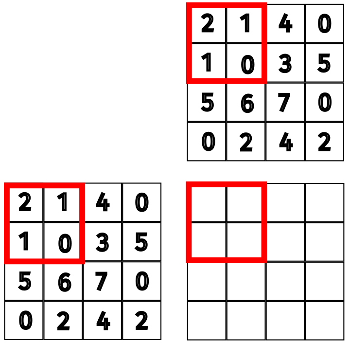
Figure 8: Setup of tiled matrix multiplication example.
The row and column of the output computed by the current thread is calculated using the block and thread indices. Of course, this is simply \((0, 0)\) for the first thread. It gets slightly more complicated when computing the input subset in the loop. The input needs to be transferred to shared memory. The loop will skip over a tile at a time. At this point, we already know which row of \(M\) and column of \(N\) we need to access. We need to compute the column index for \(M\) and the row index for \(N\).
For \(M\), we start with Row * Width. This needs to be offset by the tile offset index ph of the main loop, yielding Row * Width + ph * TILE_WIDTH. Finally, we need to add the thread index tx to get the final index Row * Width + ph * TILE_WIDTH + tx. The same process is applied to \(N\). Note that this only transfers a single value from each matrix to shared memory, but our computation relies on 2 values from each matrix. Each thread in the block is collaboratively loading the data into shared memory. This is why the call to __syncthreads() is necessary.
Specifically, the thread for \(P_{0, 0}\) copies \(M_{0, 0}\) and \(N_{0, 0}\) to shared memory. The thread for \(P_{0, 1}\) copies \(M_{0, 1}\) and \(N_{1, 0}\) to shared memory. The thread for \(P_{1, 0}\) copies \(M_{1, 0}\) and \(N_{0, 1}\) to shared memory. Finally, the thread for \(P_{1, 1}\) copies \(M_{1, 1}\) and \(N_{1, 1}\) to shared memory.
The next step is to compute the dot product of the subset. Again, we see a call to __syncthreads(). Without this synchronization, the loop may be allowed to continue and overwrite the data in shared memory before a thread has finished. Once the final value is computed, each thread can freely write it back to global memory. Since each thread is computing a different value, there is no need to synchronize the threads before writing to global memory.
\begin{align*} P_{0, 0} &+= 2 \times 2 + 1 \times 1 \\ P_{0, 1} &+= 2 \times 1 + 1 \times 0 \\ P_{1, 0} &+= 1 \times 2 + 0 \times 1 \\ P_{1, 1} &+= 1 \times 1 + 0 \times 0 \end{align*}
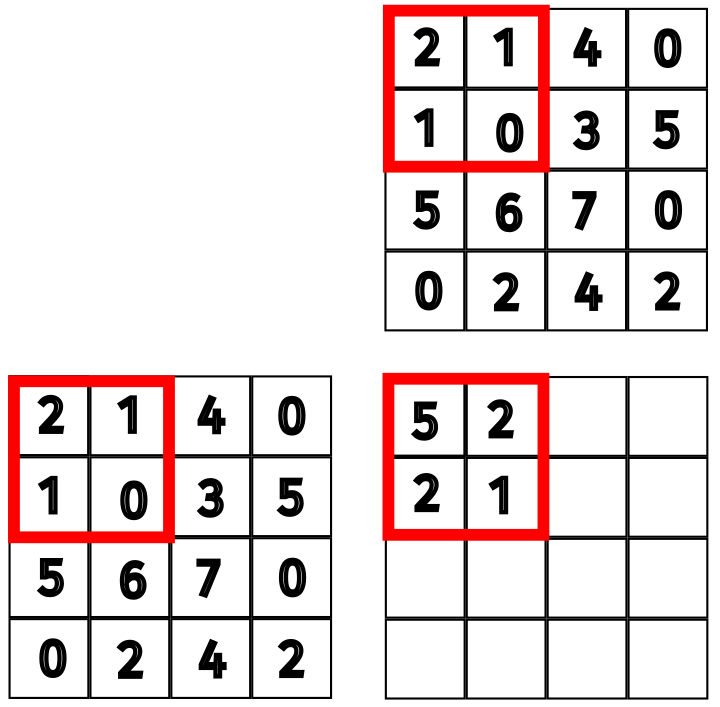
Figure 9: Updated values for the first subset.
The next iteration of the loop will grab the next subset of the data and repeat the process. The result after this step is shown below.
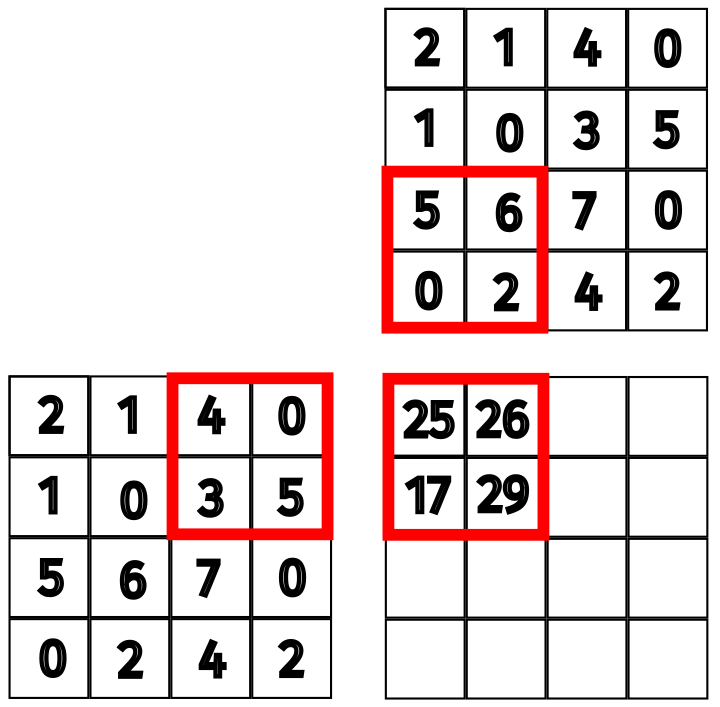
Figure 10: Updated values for the second subset.
To summarize, ph is the tile offset index, Row and Col are the row and column of the output computed by the current thread, and tx and ty will give the offset with respect to the current tile.
The kernel above has an outer loop that calls another loop managed by thread synchronization, breaking the computation up into several distinct phases. This is called strip-mining and is an important part of tiling. This existed even before GPUs were used (Hwu, Kirk, and El Hajj 2022).
Performance Analysis
In the naive implementation, we had a computational intensity of 0.25 FLOP/B. With a \(16 \times 16\) tile, the number of global memory accesses is reduced by a factor of 16. This gives us a computational intensity of 4 FLOP/B. We previously stated that the H100 has a global memory bandwidth of 3TB/s. This means that the theoretical limit for the performance of this kernel is 3000 * 4 = 12000 GFLOP/s which is much better than the 750 GFLOP/s we had before.
This is not the most optimal way to implement matrix multiplication, and you should always refer to the cuBLAS library for matrix operations. The purpose of this example is to demonstrate the use of tiling.
Boundary Checking
The previous implementation assumed that the width of the matrices was a multiple of the tile width and that the input would always be square matrices. Consider changing our \(2 \times 2\) block to a \(3 \times 3\) block using the same input sizes.
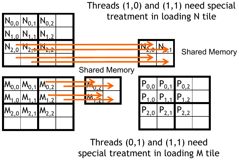
Figure 11: Using a 3x3 block (source: NVIDIA DLI).
Our implementation would follow the same process for the first subset of pattern. An issue arises when computing the second tile offset since the block exceeds the boundaries of our input and output. One solution would be to check the boundary condition on both the input, when transferring the data to shared memory, and the output, when reading the data from shared memory. This would require a conditional statement in the inner loop. This is not ideal since the conditional statement would be executed for every thread in the block.
Another solution is to pad the input with zeros. If the index is outside our boundary, adding a 0 will not affect the result of the dot product. This allows for a simpler implementation while still being flexible enough to handle matrices of any size. The relevant portion of the kernel is shown below.
float Pvalue = 0;
for (int ph = 0; ph < ceil(Width/(float)TILE_WIDTH); ph++) {
    // Collaborative loading of M and N tiles into shared memory
    if (Row < Width && ph * TILE_WIDTH + tx < Width) {
        Mds[ty][tx] = M[Row * Width + ph * TILE_WIDTH + tx];
    } else {
        Mds[ty][tx] = 0.0;
    }
    if (ph * TILE_WIDTH + ty < Width && Col < Width) {
        Nds[ty][tx] = N[(ph * TILE_WIDTH + ty) * Width + Col];
    } else {
        Nds[ty][tx] = 0.0;
    }
    __syncthreads();
}
The rest of the kernel remains the same. In Lab 2, you will implement this and adapt it to work with non square matrices as well.
Memory Use and Occupancy
Just like exceeding the number of registers per thread can negatively affect occupancy, so can over allocating shared memory. The H100 can have up to 228 KB per SM. If we are maximizing the 2048 threads available per SM, each block cannot exceed 228 KB / 2048 threads = 112 B/thread.
How much shared memory is used by each block? Each block has 2 arrays of size \(TILE\_WIDTH \times TILE\_WIDTH\) of type float. This gives us a total of \(2 \times TILE\_WIDTH \times TILE\_WIDTH \times 4 = 8(TILE\_WIDTH)^2\) B. Each block uses \(TILE\_WIDTH^2\) threads, resulting in 8 B/thread. This is well below the limit of 112 B/thread.
Dynamically Changing the Block Size
The solution presented above uses a constant to determine the tile size. What if this tile size was not optimal for a given hardware configuration? We would surely want to adjust this dynamically to maximize performance. In CUDA, we can support this by using the extern keyword. First, we need to define our shared memory as one array: extern __shared__ float Mds_Nds[];. This is a 1D array that represents the shared memory for both input matrices.
When launching this kernel, we need some way to inform it of the tile size. First, we would query the device properties and determine the optimal tile size based on the hardware. This size can be used as a third launch configuration input, as shown below. Additionally, the size of the shared memory for each input matrix is provided as two additional arguments to the kernel.
size_t size = compute_optimal_size(); // Determine optimal tile size
MatMulKernel<<<dimGrid, dimBlock, size>>>(M_d, N_d, P_d, Width, size/2, size/2);
The kernel will need to be modified to use the new shared memory array. The first step is to determine the offset for each matrix. This is done by multiplying the tile size by the thread index. The second step is to use the offset to access the correct value in the shared memory array. The kernel is shown below.
__global__ void MatMulKernel(float* M, float* N, float* P, int Width, int Mds_offset, int Nds_offset) {
    extern __shared__ float Mds_Nds[];

    float *Mds = (float *)Mds_Nds;
    float *Nds = (float *)Mds_Nds + Mds_offset;

    // Rest of the kernel
}
Completing this modification would require us to use linear indexing for Mds and Nds.
The Takeaway
Tiling is a powerful tool that can be used to improve the performance of a kernel. It is important to understand the memory access pattern of your kernel and identify which data is reused. This will allow you to move that data to shared memory and reduce the number of global memory accesses. Tiling is the first of many patterns that we will explore. Just like not every tool is useful for every job, not every pattern will be useful for each problem we face. Increasing the number of tools, or patterns, that we have available will allow us to solve a wider range of problems efficiently.