Decision Trees
Resources
Introduction
A decision tree, or Classification and Regression Trees (CART), is a model that recursively partitions the input space based on a collection of features. The partitions are split based on very simple binary choices. If yes, branch to the left; if no, branch to the right.
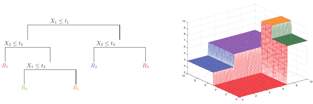
Figure 1: Regression tree (left) and its piecewise constant surface (right) (Source: Machine Learning: A Probabilistic Perspective by Kevin P. Murphy).
To compute the response, we represent each individual decision as a function \(\phi\) and sum the responses:
\[ f(\mathbf{x}) = \mathbb{E}[y | \mathbf{x}] = \sum_{m=1}^M w_m \mathbb{1} (\mathbf{x} \in R_m) = \sum_{m=1}^M w_m \phi(\mathbf{x};\mathbf{v}_m), \]
where \(R_m\) is the \(m^{\text{th}}\) region, \(w_m\) is the mean response, and \(\mathbf{v}_m\) is the choice of variable to split on along with its threshold value. Note that this is not a differentiable function due to the indicator function.
Example: Iris Dataset
To see this on real data, consider the Iris flower dataset. For example, we will look at a decision tree model that classifies each flower into either setosa, versicolor, or virginica.
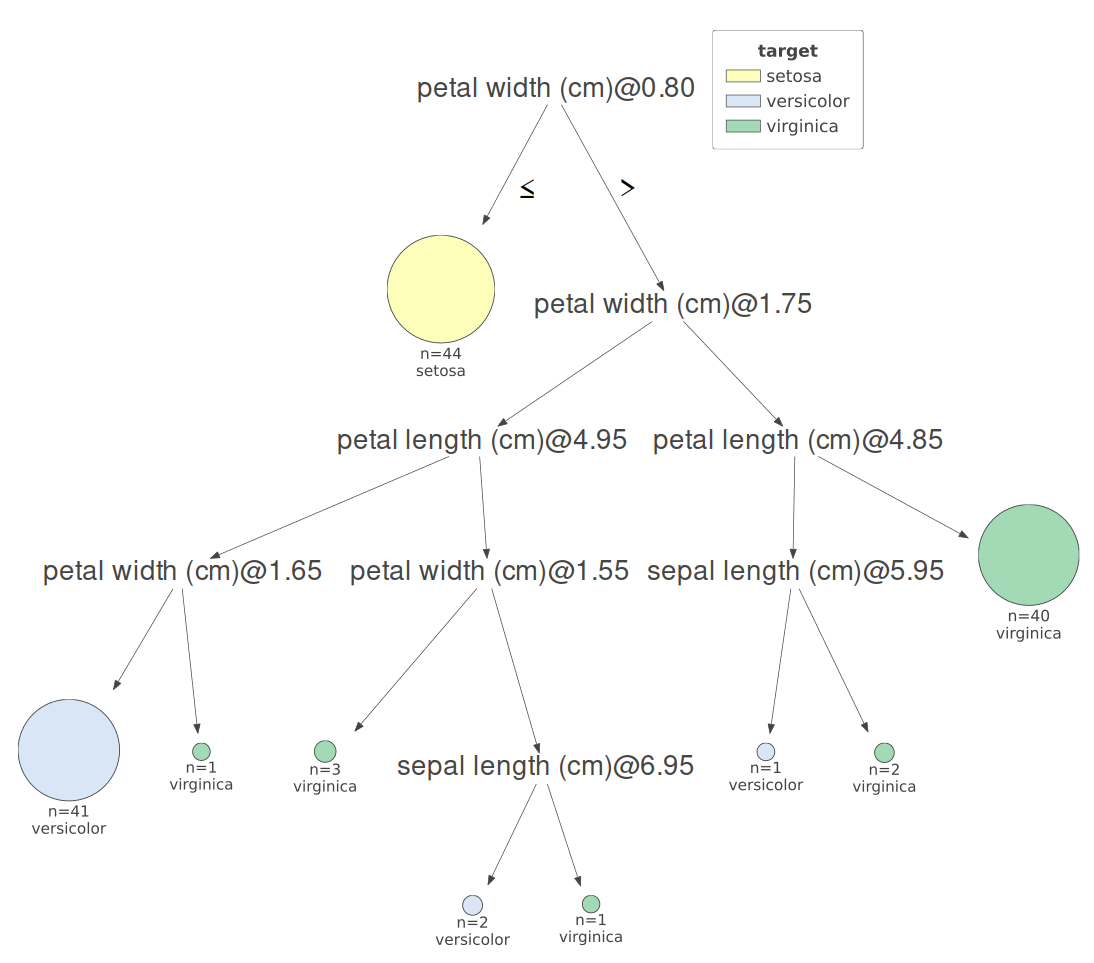
Figure 2: Our initial Iris classifier.
We are given data about a new iris and want to classify it using this tree. Our sample has a sepal length of 6.1cm, a sepal width of 2.8cm, a petal length of 4.7cm, and a petal width of 1.2cm. The first decision considers the petal width. Our sample has a width of 1.2, so it continues down the right branch.
The second decision consideres petal width again. Since our sample does not have a width greater than 1.75, we continue down the left branch.
At this point, the model was optimized to now consider the petal length. Our length comes in at 4.7, just shy of going down the right path.
We now arrive at the last decision. Since our petal length is not greater than 1.65, the model classifies this sample as versicolor.
Growing a Tree
To grow a tree, a decision needs to be made as to whether or not the current set of data can be split based on some feature. As such, there should be a reliable way of determining if a feature provided a good split. This is evaluated using a cost function and selecting the feature and value corresponding to the minimum cost:
\[ (j^*, t^*) = \text{arg} \min_{j\in\{1, \dots, D\}} \min_{t \in \mathcal{T}_j} \text{cost}(\{\mathbf{x}_i, y_i : x_{ij} \leq t\}) + \text{cost}(\{\mathbf{x}_i, y_i : x_{ij} > t\}). \]
In words, this function finds a value \(t\) such that groups the data with the lowest cost. For a regression task, the cost function is typically defined as
\[ \text{cost}(\mathcal{D}) = \sum_{i \in \mathcal{D}}(y_i - \bar{y})^2, \]
where
\[ \bar{y} = \frac{1}{|\mathcal{D}|}\sum_{i \in \mathcal{D}} y_i. \]
Splits that result in clusters with high variance may still see a higher cost, even though they are the minimum.
As their alternative name implies, decision trees can also be used for classification. The splits are still based on features and threshold values at each branch. When a split is considered, a class-conditional probability is estimated for that data.
Splitting the Data
Given a set of data that makes it to node \(i\), denoted \(\mathcal{D}_i\), a fitting procedure must select the feature and threshold value that minimizes the cost. If the feature is continuous, the range of search values is selected by sorting a list of unique values from the subset of data. For each unique value, the cost is computed by splitting the data into two groups based on the threshold value. The threshold value that minimizes the cost is selected.
In the case of categorical data, we would intuitively split the data into a set of data that contains the category and a set that does not. The cost is then computed for each category. The category that minimizes the cost is selected.
Given data satisfying \(X_j < t\), the class-conditional probability is
\[ \hat{\pi}_c = \frac{1}{|\mathcal{D}|}\sum_{i \in \mathcal{D}} \mathbb{1}(y_i = c). \]
Error Functions
The common error functions used for classification are misclassification rate, entropy, and Gini index. Misclassification rate is computed by summing the number of misclassifications:
\[ \frac{1}{|\mathcal{D}|} \sum_{i \in \mathcal{D}} \mathbb{1}(y_i \neq \hat{y}) = 1 - \hat{\pi}_{\hat{y}}. \]
Entropy is computed as
\[ \mathbb{H}(\mathbb{\hat{\pi}}) = -\sum_{c=1}^C \hat{\pi}_c \log \hat{\pi}_c. \]
Gini index computes the expected error rate.
\[ G = \sum_{c=1}^C \hat{\pi}_c (1 - \hat{\pi}_c) = 1 - \sum_{c=1}^C \hat{\pi}_c^2 \]
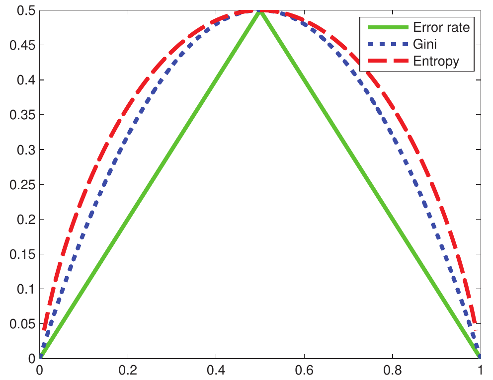
Figure 3: Impurity measured for binary classification (Source: Machine Learning: A Probabilistic Perspective by Kevin P. Murphy)
Like entropy, it promotes an equal number of observations across all classes in a node. For small values of \(\hat{\pi}\), the error is smaller than that of entropy. If the dataset is imbalanced, entropy is typically favored as it penalizes imbalanced datasets more than Gini will. Both will favor splits that result in one node being pure.
Stopping Growth
If left unchecked, the algorithm to grow a tree will continue until the data can no longer be split. In the trivial case, this will be when every data point represents a leaf node. In order to prevent overfitting, there are several criteria that are considered.
Does the split reduce the cost enough?
It may be ideal to only split the data if the cost is reduced by some acceptable value. The reduction can be computed by
\[ \Delta = \text{cost}(\mathcal{D}) - \bigg(\frac{|\mathcal{D}_L|}{|\mathcal{D}|}\text{cost}(\mathcal{D}_L) + \frac{|\mathcal{D}_R|}{|\mathcal{D}|} \text{cost}(\mathcal{D}_R)\bigg). \]
Has the tree reached some maximum depth?
The depth of a tree is set as a hyperparameter. Later, when we look at an example, we will use cross validation to select the best depth parameter for our model.
Is the distribution of the split pure?
If either of the splits is fully made up of data with the same label, there is no need to split it any further.
Is the split too small?
A split that is too small may lead to overfitting.
Examining the Iris Classification Tree
How exactly does the earlier example model make its decision at each node? The full tree is shown below.
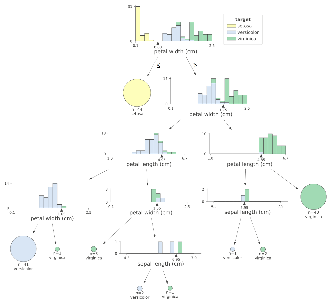
Figure 4: A detailed view of our Iris classifier.
The first split is visually very simple to intuit. Using petal width can perfectly split all setosa samples into a single leaf node.
Pruning a Tree
Depending on the data, stopping growth based on measuring the relative decrease in error may not result in a model that performs well. Image a dataset that requires multiple features to provide a sufficient classification. If only one of the features is considered in isolation, it may provide no decrease in error. A practical example of this is the XOR problem. Splitting on \(x_1\) or \(x_2\) in isolation does not provide any indication about the true output. It is only when \(x_1 \neq x_2\) does the output equal to 1.
To rectify this, a tree can be grown until it is completely full before pruning the branches that result in the smallest increase in error.
The Algorithm
The general algorithm is shown in MATLAB below.
% node = fitTree(node, D, depth)
% Recursive function to learn a decision tree
% Returns the index of the current node.
%
%   node  - The node index in obj.Nodes.
%   D     - Indices to the current data.
%   depth - Current depth of the tree.
function node = fitTree(obj, node, D, depth)
    % Determine best split for the data and return the split
    [j, t, dSplit, classDist] = obj.split(D, obj.Nodes(node).features);
    obj.Nodes(node).prediction = classDist;
    disp(classDist);

    % Use heuristic to determine if node is worth splitting
    if obj.splitNode(depth, classDist) == true
        % set the node test, the function that determines the branch
        obj.Nodes(node .test = {j, t};
        newFeatures = obj.Nodes(node).features(obj.Nodes(node).features ~= j);

        % set the child nodes to the left and right splits
        obj.Nodes(node).children = zeros(size(dSplit, 1), 1);
        numNewNodes = size(dSplit, 1);
        for i = 1 : numNewNodes
            obj.Nodes(end + 1) = struct('prediction', 0, 'test', 0, ...
                'features', newFeatures, 'children', 0, 'parent', node);
            obj.Nodes(node).children(i)  = obj.fitTree(length(obj.Nodes), dSplit{i}, depth + 1);
        end
    end
end