Deep Learning
Introduction
Deep learning is a term that you’ve probably heard of a million times by now in different contexts. It is an umbrella term that encompasses techniques for computer vision, bioinformatics, natural language processing, and much more. It almost always involves a neural network of some kind that was trained on a large corpus of data.
The existence of the word “deep” implies a contrast to “shallow” learning. Some definition define a deep network as an artificial neural network with more than 1 layer. Another definition is that a deep model will include a hierarchy of features that are learned from the data. These features are learned as part of the optimization process as opposed to being manually engineered as is required in other machine learning techniques.
If you are not yet familiar with neural networks, follow the link to learn about their basics as they are the foundation of deep learning systems.
We will cover how to implement an array of deep learning models for different tasks. Different layers and activation functions will be explored as well as the effect of regularization. There will also be a focus on best practices for organizing a machine learning project.
What makes a model deep?
We begin by comparing shallow networks with deep networks. What defines a deep network? Is it as simple as crossing a threshold into \(n\) layers? As evidenced by (Zeiler and Fergus 2013) deeper networks allow for a more robust hierarchy of image features.
There is work by (Montúfar et al. 2014) which suggests that shallow networks require an exponential amount of nodes as compared to deeper networks. Additionally, there are many individual results which suggest that deeper networks provide better task generalization.
As we will later see when studying Convolutional Neural Networks, the optimization of such deep networks produces features that maximize the performance of a task. That is, the network is not only optimizing the overall performance of task, but it produces features from the data that may be useful in other contexts. This is particularly useful for transfer learning, where large pre-trained models can be used as starting points for novel tasks. The benefit being that a complete retraining of the model is not necessary.
Deep Networks
Like neural networks, deep networks are defined by the number of layers, nodes per layer, activation functions, and loss functions. We now review the forward and backward pass, providing more insight into the structure and usage of deep networks along the way.
Consider a deep network with \(L\) layers. Layer \(l\) has \(n_{l-1}\) input connections and \(n_l\) output nodes and activation function \(g^{(l)}\). The final output is evaluated with some ground truth using a loss function \(\mathcal{L}\).
Forward Pass
\begin{align*} \mathbf{a}^{(l)} &= W^{(l)}\mathbf{z}^{(l-1)} + \mathbf{b}^{(l)}\\ \mathbf{z}^{(l)} &= g^{(l)}(\mathbf{a}^{(l)})\\ \end{align*}
This is repeated from the input to the last layer. For the first layer \(l=1\), the input \(\mathbf{z}^{(0)} = \mathbf{x}\). In practice, the output \(\mathbf{a}^{(l)}\) is cached since it is required for the backward pass. This prevents the values from needing to be computed twice.
It is also worth it to study the sizes of the matrices while performing a forward pass. For a layer \(l\), \(W^{(l)} \in \mathbb{R}^{n_l \times n_{l-1}}\) and the input \(\mathbf{z}^{(l-1)} \in \mathbb{R}^{n_{l-1} \times 1}\). When training, it is common to perform batch gradient descent with batches of input of size \(B\). Then, \(\mathbf{z}^{(l-1)} \in \mathbb{R}^{n_{l-1}\times B}\) and \(\mathbf{a}^{(l)}, \mathbf{b}^{(l)} \in \mathbb{R}^{n_l \times B}\).
Backward Pass
During the backward pass, the gradient is propagated from the last layer to the first. Each layer that contains trainable parameters must also compute the gradient of the network output with respect to the weights and biases. This can be done in a modular way, as shown next.
Consider the last layer. The gradients with respect to the weights and biases are
\begin{align*} \frac{d\mathcal{L}}{dW^{(L)}} &= \frac{d\mathcal{L}}{d\mathbf{z}^{(L)}} \frac{d\mathbf{z}^{(L)}}{d\mathbf{a}^{(L)}} \frac{d\mathbf{a}^{(L)}}{dW^{(L)}}\\ \frac{d\mathcal{L}}{d\mathbf{b}^{(L)}} &= \frac{d\mathcal{L}}{d\mathbf{z}^{(L)}} \frac{d\mathbf{z}^{(L)}}{d\mathbf{a}^{(L)}} \frac{d\mathbf{a}^{(L)}}{d\mathbf{b}^{(L)}}. \end{align*}
To see how the gradient continues to be propagated backward, compute the same thing for layer \(L-1\)
\begin{align*} \frac{d\mathcal{L}}{dW^{(L-1)}} &= \frac{d\mathcal{L}}{d\mathbf{z}^{(L)}} \frac{d\mathbf{z}^{(L)}}{d\mathbf{a}^{(L)}} \frac{d\mathbf{a}^{(L)}}{d\mathbf{z}^{(L-1)}} \frac{d\mathbf{z}^{(L-1)}}{d\mathbf{a}^{(L-1)}} \frac{d\mathbf{a}^{(L-1)}}{dW^{(L-1)}}\\ \frac{d\mathcal{L}}{d\mathbf{b}^{(L-1)}} &= \frac{d\mathcal{L}}{d\mathbf{z}^{(L)}} \frac{d\mathbf{z}^{(L)}}{d\mathbf{a}^{(L)}} \frac{d\mathbf{a}^{(L)}}{d\mathbf{z}^{(L-1)}} \frac{d\mathbf{z}^{(L-1)}}{d\mathbf{a}^{(L-1)}} \frac{d\mathbf{a}^{(L-1)}}{d\mathbf{b}^{(L-1)}}. \end{align*}
As seen above, to continue propagating the gradient backward, each layer \(l\) must also compute
\[ \frac{d\mathbf{a}^{(l)}}{d\mathbf{z}^{(l-1)}}. \]
To summarize, every layer with trainable parameters will compute
\begin{align*} \frac{d\mathcal{L}}{dW^{(l)}} = \frac{d\mathbf{a}^{(l+1)}}{d\mathbf{z}^{(l)}} \frac{d\mathbf{z}^{(l)}}{d\mathbf{a}^{(l)}} \frac{d\mathbf{a}^{(l)}}{dW^{(l)}}\\ \frac{d\mathcal{L}}{d\mathbf{b}^{(l)}} = \frac{d\mathbf{a}^{(l+1)}}{d\mathbf{z}^{(l)}} \frac{d\mathbf{z}^{(l)}}{d\mathbf{a}^{(l)}} \frac{d\mathbf{a}^{(l)}}{d\mathbf{b}^{(l)}}. \end{align*}
The term \(\frac{d\mathbf{a}^{(l+1)}}{d\mathbf{z}^{(l)}}\) is the gradient that is propagated from layer \(l+1\).
Deep vs. Shallow Networks
As mentioned above, a shallow network can approximate any continuous function to arbitrary precision. If a deep network can represent the composition of two shallow networks, then it can also approximate any continuous function to arbitrary precision. Then why are deep networks better than shallow networks when both can approximate any function? There are a few compelling reasons as to why, starting with the capacity of the network and the number of linear regions it can represent per parameter.
As discussed in Understanding Deep Learning (Prince 2023), a shallow network with 1 input, 1 output, and \(D > 2\) hidden units can create up to \(D + 1\) linear regions using \(3D+1\) parameters. The \(3D + 1\) comes from the fact that the hidden layer requires \(D\) parameters for the weights with an extra \(D\) parameters for the bias terms. To convert from the hidden layer to the output layer, there are \(D\) parameters for the weights and 1 parameter for the bias term. The figure below shows the maximum number of linear regions as a function of the number of parameters for networks that map one input to one output.
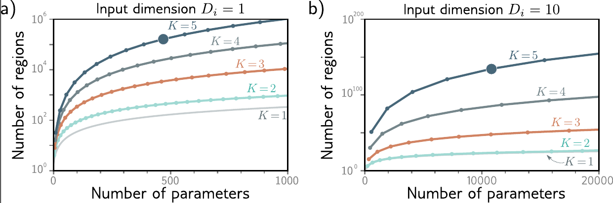
Figure 1: Maximum number of linear regions as a function of the number of parameters for networks that map one input to one output (Prince 2023).
High Dimensional Structured Data
For high dimensional structured data, such as images, deep networks are able to learn a hierarchy of features that are useful for the task at hand while requiring a significantly smaller number of parameters than a shallow network. Consider a \(100\times100\) image used as input to a shallow network with 1 hidden layer. This would require \(10,001\) parameters to represent the weights and biases. If we instead use a deep network with with convolutional layers, we can use significantly fewer parameters. We will see this more closely when we study Convolutional Neural Networks.
Activation Functions
Sigmoid
Function
\[ \sigma(\mathbf{x}) = \frac{1}{1 + \exp(-\mathbf{x})} \]
Derivative
\[ \sigma(\mathbf{x})(1 - \sigma(\mathbf{x})) \]
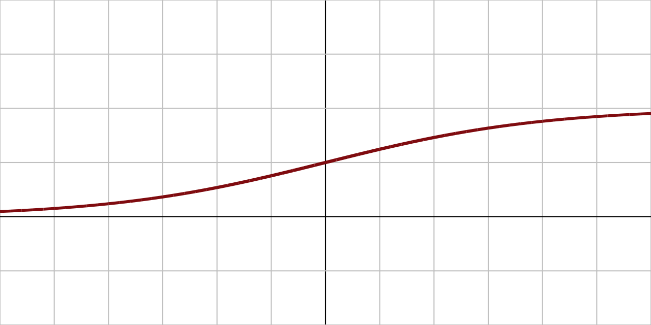
Figure 2: Sigmoid non-linearity (Wikipedia)
Loss Functions
Loss functions are used to evaluate the performance of a model. In the context of gradient descent, their gradient with respect to the model parameters is used to update the parameters. Loss functions can be constructed using maximum likelihood estimation over a probability distribution or by using a distance metric between the model output and the ground truth. The table below from (Prince 2023) shows some common loss functions and their use cases.
| Data Type | Domain | Distribution | Use |
|---|---|---|---|
| Univariate, continuous, unbounded | \(\mathbb{R}\) | univariate normal | Regression |
| Univariate, discrete, binary | \(\{0, 1\}\) | Bernoulli | Binary Classification |
| Univariate, discrete, bounded | \(\{0, 1\}^K\) | Multinoulli | Multiclass Classification |
A Typical Training Pipeline
When training and evaluating models, especially on benchmark datasets, it is important to properly test their generalization performance. This test is crucial when comparing the efficacy of your ideas versus baseline evaluations or competing methods.
To ensure that your model is evaluated in a fair way, it is common to set aside a set of test data that is only used during the final comparison. This data is typically annotated so that some metric can be used.
It is true that the training data drives the parameter tuning during optimization. This is most commonly done with gradient descent. However, we will also change the hyperparamers such as learning rate, batch size, and data augmentation. In this case, we want to evaluate the relative performance of each change.
If we use the test set to do this, then we are necessarily using the test set for training. Our biases and intuitions about the model’s performance would be implicitly influenced by that set. To track our relative changes without using the test set, we can take a portion of the original training set and label it as our validation set.
The split between training, validation, and test data is relatively small. Most modern datasets are large, with millions of samples. Consider ImageNet, an image classification dataset with over 14 million samples. Taking 10,000 samples to serve as a validation set is only \(~.07\%\) of the dataset.
Most modern machine learning frameworks have an easy way to split the dataset.
We can do this in PyTorch using torch.utils.data.random_split.
train_dataset, val_dataset = torch.utils.data.random_split(dataset, [train_size, val_size])