Discriminant Functions
Introduction
The notebook for this lesson can be found here.
With linear regression, we were able to fit a model to our data in order to make inferences on unseen data points. In the examples, both the input features and observation were continuous. With discriminant functions, we will use similar models to classify the data points based on their input features. We start out with the simplest approach: we assume that the data is linearly separable and can be assigned one of \(K\) discrete classes.
For classification with linear discriminant functions, we will use a \(K\) dimensional vector that has a 1 corresponding to the class encoding for that input and a 0 for all other positions. For example, if our possible target classes were \(\{\text{car, truck, person}\}\), then a target vector for \(\text{person}\) would be \(\mathbf{y} = [0, 0, 1]^T\).
This article will stick to a discriminative approach to classification. That is, we define a discriminant function which assigns each data input \(\mathbf{x}\) to a class. For a probabilistic perspective, see Linear Discriminant Analysis.
We will again start with a linear model \(y = f(\mathbf{x}; \mathbf{w})\). Unlike the model used with linear regression, ours will need to predict a discrete class label. In other words, we need to predict a vector with a 1 corresponding to the class encoding.
Binary Classification
Consider a simple dataset with 2 features per data sample. Our goal is to classify the data as being one of two possible classes. This only requires a single function which classifies the sample as being in class 0 if \(f(\mathbf{x};\mathbf{w}) \geq 0\) and class 1 otherwise.
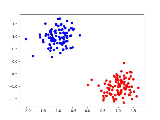
Figure 1: Two groups of data that are very clearly linearly separable.
The model output is such that \(f(\mathbf{x};\mathbf{w}) = [1, 0]\) when \(\mathbf{x}\) is predicted as class 1. If \(f(\mathbf{x};\mathbf{w}) = [0, 1]\) then \(\mathbf{x}\) is assigned to class 2. In practice, the actual output will not be a one-hot vector. There will be some values in all positions of the vector.
For example, a model trained on a binary classification task outputs the following vector given a randomly selected input sample:
\[ [0.1224, 0.8776] \]
A class would be assigned by taking the argmax of this output vector. That is, the model predicts that this sample belongs to class 1.
Measuring Classifier Performance
L1 loss can be used to measure classifier performance for linear discriminant function models.
\[ E = \sum_{i=1}^N \sum_{j=1}^M |\hat{y}_{ij} - y_{ij}| \]
Plotting a Decision Boundary
In the case of binary classification, a sample is predicted as class 1 if the output vector has the highest value at index 0. Otherwise, it is classified as class 2. If we were to plot the decision regions, we would see that the boundary is at the point when the output for both classes is equal.
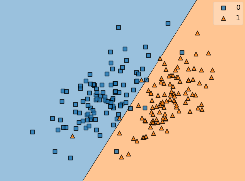
Figure 2: Binary classification with decision regions shown.
Multiple Classes
Extending this to multiple classes is as easy as encoding the classes in a one-hot vector whose length equals the number of classes. The parameters of the model can be obtained using gradient descent, the normal equations, or any other method that optimizes the least squares criterion.
The figure below shows an example of a linear discriminant function model fit to a dataset with 3 classes.
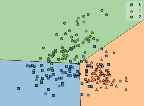
Figure 3: Multiclass classification using linear discriminant functions.
Sensitivity to Outliers
One major flaw with least squares models is their sensitivity to outliers in the data. Consider the dataset shown below.
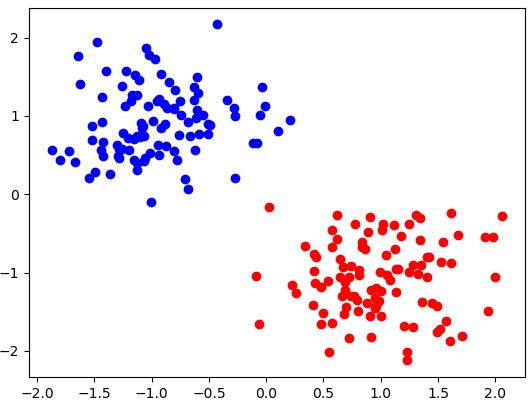
Figure 4: Linearly separable dataset
This dataset is clearly linearly separable. This will be no problem for our linear classifier, as seen below.
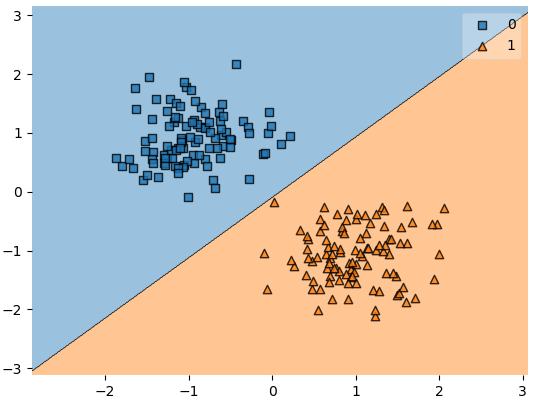
Figure 5: Linear classifier fit to data using least squares.
This dataset has a convenient property that the samples from each class are tightly clustered. What happens if our data is slightly more diverse?
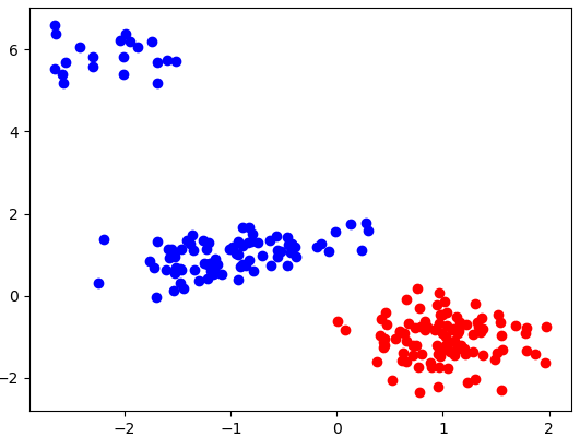
Figure 6: 2-class dataset in which one class is not as tightly clustered as the other.
In the dataset above, we can still clearly see that it should be linearly separable. Unfortunately, our least squares model will be very sensitive to the 20 points at the top left of the plot. Training a linear discriminant function using least squares results in the following decision boundary.
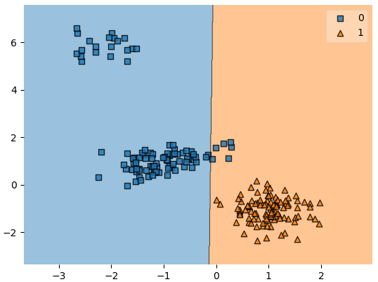
Figure 7: The model misclassifies samples that should be linearly separable.
If we determine that a linear classifier is adequate for a given dataset, we may wish to use a slightly more robust model such as Logistic Regression instead of linear discriminant functions.