Divide and Conquer Algorithms
The lecture slides for these notes are available here.
Definition
Divide and conquer algorithms are a class of algorithms that solve a problem by breaking it into smaller subproblems, solving the subproblems recursively, and then combining the solutions to the subproblems to form a solution to the original problem. Problems that can be solved in this manner are typically highly parallelizable. These notes investigate a few examples of classic divide and conquer algorithms and their analysis.
A divide and conquer method is split into three steps:
- Divide the problem into smaller subproblems.
- Conquer the subproblems by solving them recursively.
- Combine the solutions to the subproblems to form a solution to the original problem.
Their runtime can be characterized by the recurrence relation \(T(n)\). A recurrence \(T(n)\) is algorithmic if, for every sufficiently large threshold constant \(n_0 > 0\), the following two properties hold:
- For all \(n \leq n_0\), the recurrence defines the running time of a constant-size input.
- For all \(n \geq n_0\), every path of recursion terminates in a defined base case within a finite number of recursive calls.
The algorithm must output a solution in finite time. If the second property doesn’t hold, the algorithm is not correct – it may end up in an infinite loop.
“Whenever a recurrence is stated without an explicit base case, we assume that the recurrence is algorithmic.” (Cormen et al. 2022).
This assumption means that the algorithm is correct and terminates in finite time, so there must be a base case. The base case is less important for analysis than the recursive case. For example, your base case might work with 100 elements, and that would still be \(\Theta(1)\) because it is a constant.
It is common to break up each subproblem uniformly, but it is not always the best way to do it. For example, an application such as matrix multiplication is typically broken up uniformly since there is no spatial or temporal relationship to consider. Algorithms for image processing, on the other hand, may have input values that are locally correlated, so it may be better to break up the input in a way that preserves this correlation.
Solving Recurrences
- Substitution method
- Recursion-tree method
- Master method
- Akra-Bazzi method
Example: Merge Sort
Merge sort is a classic example of a divide and conquer algorithm. It works by dividing the input array into two halves, sorting each half recursively, and then merging the two sorted halves.
Divide
The divide step takes an input subarray \(A[p:r]\) and computes a midpoint \(q\) before partitioning it into two subarrays \(A[p:q]\) and \(A[q+1:r]\). These subarrays will be sorted recursively until the base case is reached.
Conquer
The conquer step recursively sorts the two subarrays \(A[p:q]\) and \(A[q+1:r]\). If the base case is such that the input array has only one element, the array is already sorted.
Combine
The combine step merges the two sorted subarrays to produce the final sorted array.
Python Implementation
def merge_sort(A):
    if len(A) <= 1:
        # Conquer -- base case
        return A

    # Divide Step
    mid = len(A) // 2
    left = merge_sort(A[:mid])
    right = merge_sort(A[mid:])

    # Combine Step
    return merge(left, right)


def merge(left, right):
    result = []
    i, j = 0, 0

    # Merge the two subarrays
    while (i < len(left)) and (j < len(right)):
        if left[i] < right[j]:
            result.append(left[i])
            i += 1
        else:
            result.append(right[j])
            j += 1

    # Add the remaining elements to the final array
    result += left[i:]
    result += right[j:]
    return result
This function assumes that the subarrays left and right are already sorted. If the value in the left subarray is less than the value in the right subarray, the left value is added to the final array. Otherwise, the right value is added. As soon as one of the subarrays is exhausted, the remaining elements in the other subarray are added to the final array. This is done with slicing in Python.
The divide step simply splits the data into left and right subarrays. The conquer step simplifies the sorting process by reducing it down to the base case – a single element. Finally, the combine step merges or folds the two sorted subarrays together.
Example code can be found here.
Analysis
When analyzing the running time of a divide and conquer algorithm, it is safe to assume that the base case runs in constant time. The focus of the analysis should be on the recurrence equation. For merge sort, we originally have a problem of size \(n\). We then divide the problem into 2 subproblems of size \(n/2\). Therefore the recurrence is \(T(n) = 2T(n/2)\). This recurrence continues for as long as the base case is not reached.
Of course we also have to factor in the time it takes for the divide and combine steps. These can be represented as \(D(n)\) and \(C(n)\), respectively. The total running time of the algorithm is then \(T(n) = 2T(n/2) + D(n) + C(n)\) when \(n >= n_0\), where \(n_0\) is the base case.
For merge sort specifically, the base case is \(D(n) = \Theta(1)\) since all it does is compute the midpoint. As we saw above, the conquer step is the recurrence \(T(n) = 2T(n/2)\). The combine step is \(C(n) = \Theta(n)\) since it takes linear time to merge the two subarrays. Thus, the worst-case running time of merge sort is \(T(n) = 2T(n/2) + \Theta(n)\).
Not every problem will have a recurrence of \(2T(n/2)\). We can generalize this to \(aT(n/b)\), where \(a\) is the number of subproblems and \(b\) is the size of the subproblems.
We haven’t finished the analysis yet since it is still not clear what the asymptotic upper bound is. Recurrence trees can be used to visualize the running time of a divide and conquer algorithms. After inspecting the result of the tree, we will be able to easily determine the complexity of merge sort in terms of big-O notation.
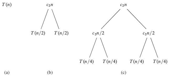
Figure 1: Expansion of recursion tree for merge sort (Cormen et al. 2022).
In the figure above from Introduction to Algorithms, the root of the tree represents the original problem of size \(n\) in (a). In (b), the divide step splits the problem into two problems of size \(n/2\). The cost of this step is indicated by \(c_2n\). Here, \(c_2\) represents the constant cost per element for dividing and combining. As mentioned above, the combine step is dependent on the size of the subproblems, so the cost is \(c_2n\). Subfigure (c) shows a third split, where each new subproblem has size \(n/4\). This would continue recursively until the base case is reached, as shown in the figure below.
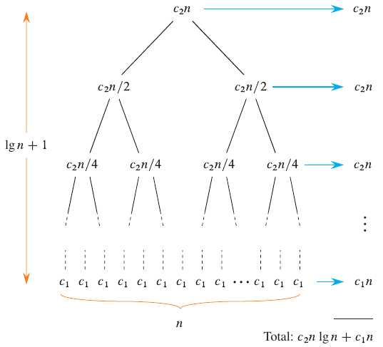
Figure 2: Full recursion tree for merge sort (Cormen et al. 2022).
The upper bound for each level of the tree is \(c_2n\). The height of a binary tree is \(\log_b n\). The total cost of the tree is the sum of the costs at each level. In this case, the cost is \(c_2n \log n + c_1n\), where the last \(c1_n\) comes from the base case. The first term is the dominating factor in the running time, so the running time of merge sort is \(\Theta(n \log n)\).
Questions
- Assume that the base case is \(n > 1\). What is the running time of the conquer step dependent on?
Example: Multiplying Square Matrices
Matrix multiplication is defined as follows:
def square_matrix_multiply(A, B):
    n = len(A)
    C = [[0 for _ in range(n)] for _ in range(n)]
    for i in range(n):
        for j in range(n):
            for k in range(n):
                C[i][j] += A[i][k] * B[k][j]
    return C
Initializing values takes \(\Theta(n^2)\). The full process takes \(\Theta(n^3)\).
Divide and Conquer
In this approach, the matrix will be split into block matrices of size \(n/2\). Each submatrix can be multiplied with the corresponding submatrix of the other matrix. The resulting submatrices can be added together to form the final matrix. This is permissible based on the definition of matrix multiplication.
Base case is \(n=1\) where only a single addition and multiplication are performed. This is \(T(1) = \Theta(1)\). For \(n > 1\), the recursive algorithm starts by splitting into 8 subproblems of size \(n/2\). There are 8 subproblems because there are 4 submatrices in each matrix, and each submatrix is multiplied with the corresponding submatrix in the other matrix.
Each recursive call contributes \(T(n/2)\) to the running time. There are 8 recursive calls, so the total running time is \(8T(n/2) + \Theta(n^2)\). There is no need to implement a combine step since the matrix is updated in place. The final running time is \(T(n) = 8T(n/2) + \Theta(1)\) for the recursive portion.
This method easily adapts to parallel processing. The size of each tile can be adjusted to fit the number of processors available. The algorithm can be parallelized by assigning each processor to a subproblem.
We now walk through an example on a \(4 \times 4\) matrix. Assume that each \(A_{ij}\) and \(B_{ij}\) is a \(2 \times 2\) matrix.
\begin{bmatrix} A_{11} & A_{12} \\ A_{21} & A_{22} \end{bmatrix}
\begin{bmatrix} B_{11} & B_{12} \\ B_{21} & B_{22} \end{bmatrix}
These matrices are already partitioned. They currently don’t meet the base case, so 8 recursive calls are made which compute the following products:
- \(A_{11}B_{11}\)
- \(A_{12}B_{21}\)
- \(A_{11}B_{12}\)
- \(A_{12}B_{22}\)
- \(A_{21}B_{11}\)
- \(A_{22}B_{21}\)
- \(A_{21}B_{12}\)
- \(A_{22}B_{22}\)
Peeking into the first recursive call, the \(2 \times 2\) matrices are partitioned into 4 \(1 \times 1\) matrices, or scalars. The base case is reached, and the product is computed. The same process is repeated for the other 7 recursive calls. The final matrix is then formed by adding the products together.
def partition(A):
    n = len(A)
    mid = n // 2
    A11 = [row[:mid] for row in A[:mid]]
    A12 = [row[mid:] for row in A[:mid]]
    A21 = [row[:mid] for row in A[mid:]]
    A22 = [row[mid:] for row in A[mid:]]
    return A11, A12, A21, A22

def matrix_multiply_recursive(A, B, C, n):
    if n == 1:
        C[0][0] += A[0][0] * B[0][0]
    else:
        # Partition the matrices
        A11, A12, A21, A22 = partition(A)
        B11, B12, B21, B22 = partition(B)
        C11, C12, C21, C22 = partition(C)

        # Recursively compute the products
        matrix_multiply_recursive(A11, B11, C11, n/2)
        matrix_multiply_recursive(A12, B21, C11, n/2)
        matrix_multiply_recursive(A11, B12, C11, n/2)
        matrix_multiply_recursive(A12, B22, C11, n/2)
        matrix_multiply_recursive(A21, B11, C11, n/2)
        matrix_multiply_recursive(A22, B21, C11, n/2)
        matrix_multiply_recursive(A21, B12, C11, n/2)
        matrix_multiply_recursive(A22, B22, C11, n/2)
Analysis
Each recursive call contributes \(T(n/2)\) to the running time. Unless the base case is reached, each call contributes 8 recursive calls to the recurrence, yielding a running time of \(T(n) = 8T(n/2) + \Theta(1)\).
Example: Convex Hull
Given \(n\) points in plane, the convex hull is the smallest convex polygon that contains all the points.
-
No two points have the same \(x\) or \(y\) coordinate.
-
Sequence of points on boundary in clockwise order as doubly linked list.
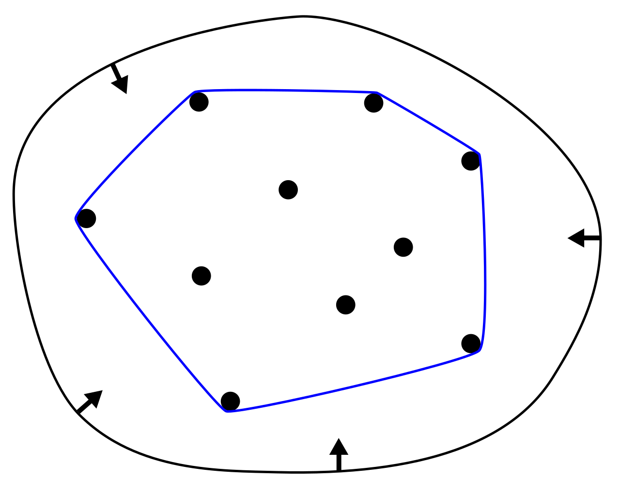
Figure 3: Convex Hull (source: Wikipedia)
Naive Solution
Draw lines between each pair of points. If all other points are on the same side of the line, the line is part of the convex hull. This is \(\Theta(n^3)\).
Divide and Conquer
Sort the points by \(x\) coordinate. Split into two halves by \(x\). Recursively find the convex hull of each half. Merge the two convex hulls.
Merging
Find upper tangent and lower tangent.
Why not just select the highest point from each half?
The highest point in each half may not be part of the convex hull. The question assumes that the two convex hulls are relatively close to each other.
Two Finger Algorithm
Start at the rightmost point of the left convex hull and the leftmost point of the right convex hull. Move the right finger clockwise and the left finger counterclockwise until the tangent is found. The pseudocode is as follows:
def merge_convex_hulls(left, right):
    # Find the rightmost point of the left convex hull
    left_max = max(left, key=lambda p: p[0])
    # Find the leftmost point of the right convex hull
    right_min = min(right, key=lambda p: p[0])
    # Find the upper tangent
    while True:
        # Move the right finger clockwise
        right_max = max(right, key=lambda p: p[0])
        if is_upper_tangent(left_max, right_max):
            break
        # Move the left finger counterclockwise
        left_max = max(left, key=lambda p: p[0])
    # Find the lower tangent
    while True:
        # Move the right finger clockwise
        right_min = min(right, key=lambda p: p[0])
        if is_lower_tangent(left_min, right_min):
            break
        # Move the left finger counterclockwise
        left_min = min(left, key=lambda p: p[0])
This runs in \(\Theta(n)\) time.
Removing the lines that are not part of the convex hull require the cut and paste operations. Starting at the upper tangent, move clockwise along the right convex hull until you reach the point in the lower tangent of the right convex hull. Make the connection to the corresponding point on the left convex hull based on the lower tangent, then move clockwise until you reach the upper tangent of the left convex hull. This is \(\Theta(n)\).
Orientation Test
The orientation test is a technique from computational geometry which determines the orientation of three points. For our purposes, it will tell us if a third point lies below or above a given line segment. The orientation test is used to determine if a point is part of the convex hull.
Given three points \(p\), \(q\), and \(r\), the orientation is determined by the sign of the cross product of the vectors \(\overrightarrow{pq}\) and \(\overrightarrow{pr}\). If the cross product is positive, the orientation is clockwise. If the cross product is negative, the orientation is counterclockwise. If the cross product is zero, the points are collinear.
This is expressed by a simple formula:
\[ \text{orientation}(p, q, r) = (q_y - p_y)(r_x - q_x) - (q_x - p_x)(r_y - q_y) \]
Consider the visualization below. Let \(p\) be a point in the left convex hull and \(q\) be a point in the right convex hull. The orientation test will tell us if \(r\) is above or below the line segment \(\overline{pq}\). If the test is negative, \(r\) is above the line segment and is part of the convex hull, and vice versa.
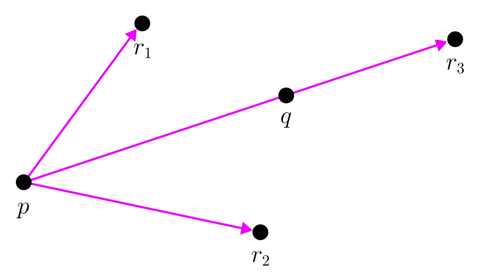
Figure 4: Visualization of the orientation test.
When checking to see if a line is an upper tangent, consider the points \(p\), \(q\), and \(r\), where \(p\) is from the left convex hull and \(q\) is from the right convex hull. Let \(r\) be the point immediately after \(q\) in a clockwise direction.
Example: Median Search
Finding the median value of a set can be performed in linear time without fully sorting the data. The recurrence is based on discarding a constant fraction of the elements at each step.
Algorithm
- Divide: Partition the set into groups of 5 elements. Depending on the size of the set, there may be less than 5 elements in the last set.
- Conquer: Sort each group and find the median of each group. Since the subsets are of constant size, this is done in constant time.
- Combine: Given the median of each group from step 2, find the median of medians. This value will be used as a pivot for the next step.
- Partition: Use the pivot to separate values smaller and larger than the pivot.
- Select: If the given pivot is the true median based on its position in the original set, select it. If not, recursively select the median from the appropriate partition.
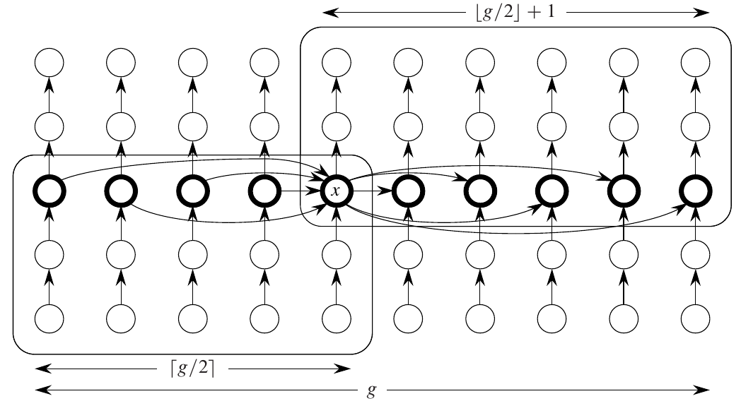
Figure 5: Visualization of median of medians (Cormen et al. 2022).
Given a set of \(n\) numbers, define \(rank(X)\) as the number in the set that are less than or equal to \(X\).
\(Select(S, i)\)
- Pick \(x \in S\)
- Compute \(k = rank(x)\)
- B = {y in S | y < x}
- C = {y in S | y > x}
If \(i = k\), return \(x\). else if \(k > i\), return \(Select(B, i)\). else return \(Select(C, i-k)\).
How do we get balanced partitions?
Arrange \(S\) into columns of size 5. Sort each column descending (linear time). Find “median of medians” as \(X\)
If the columns are sorted, it is trivial to find the median of each column.
Half of the groups contribute at least 3 elements greater than \(X\), except for the last group. We have one group that contains \(x\).
Analysis
Given a set \(A = \{a_1, a_2, \ldots, a_n\}\), the median search algorithm returns the $k$th smallest element of \(A\). We now analyze the runtime of this algorithm.
Divide
In the divide step, the set is partitioned into \(\lceil n/5 \rceil\) groups of 5 elements each. This is done in linear time.
Conquer
Each group is sorted using insertion sort or some other algorithm. Even though the search itself may have a higher complexity, the sorting of the groups is \(\Theta(1)\) since the groups are of constant size. Collectively across all groups, the sorting is \(\Theta(n)\).
Combine
The median of each group is found, introducing a recurrence of \(T(\lceil n/5 \rceil)\). Once each median is found, the median of medians is computed.
Partition
As reasoned above, the median of medians is used as a pivot to partition the set into two groups. At least 30% of the elements are greater than the pivot. This leaves a search space of at most \(7n/10\). Partitioning is done in linear time.
Select
If the pivot is the $k$th smallest element, the algorithm terminates. Otherwise, the algorithm recursively searches the appropriate partition. Comparing the size of the partition to the size of the original set, the recurrence is \(T(7n/10)\).
Pseudocode is available here.