Dynamic Programming
The slides for these lectures notes can be found here.
Dynamic programming is a technique for solving problems by breaking them down into simpler subproblems, very much like divide and conquer algorithms. One primary difference is that the subproblems are designed in such a way that they do not need to be recomputed.
Many common problems have efficience dynamic programming solutions, and we will investigate several of them in these notes. In general, a dynamic programming solution can be applied if the problem has the following features.
- Optimal substructure: An optimal solution can be constructed by optimal solutions to the subproblems.
- Overlapping subproblems: The problem can be broken down into subproblems which can be reused.
For example, the Fibonacci sequence has optimal substructure because the value of the sequence at any index is the sum of the values at the two previous indices. It also has overlapping subproblems because the value of the sequence at any index is used in the calculation of the values at the two subsequent indices. A recursive solution to the Fibonacci sequence will have exponential time complexity, but a dynamic programming solution will have linear time complexity.
The two main approaches to dynamic programming are top-down (memoization) and bottom-up (tabulation). Memoization involves writing a recursive solution that stores each sub=solution in a table so that it can be reused. Tabulation involves solving the problem by filling in a table of subproblems from the bottom up. In either case, a dynamic programming solution can be formulated with the following steps.
- Identify subproblems so that the problem can be broken down.
- Solve the subproblems following an optimal solution.
- Store the solutions to avoid redundant computation.
- Combine solutions from the subproblems to solve the original problem.
Rod Cutting
Given a rod of length \(n\) and table of prices \(p_i\) for \(i = 1, 2, \ldots, n\), determine the maximum revenue \(r_n\) that can be obtained by cutting up the rod and selling the pieces.
| Length | 1 | 2 | 3 | 4 | 5 | 6 | 7 | 8 | 9 | 10 |
|---|---|---|---|---|---|---|---|---|---|---|
| Price | 1 | 5 | 8 | 9 | 10 | 17 | 17 | 20 | 24 | 30 |
The table of prices is shown above. For a rod of length 4, there are 8 (\(2^{n-1}\), where \(n=4\)) different ways to cut the rod.
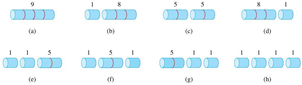
Figure 1: 8 different ways to cut a rod of length 4 (Cormen et al. 2022).
The maximum revenue for a rod of length \(n\) can be determined by the following optimization problem:
\[ r_n = \max(p_n, r_1 + r_{n-1}, r_2 + r_{n-2}, \ldots, r_{n-1} + r_1), \]
where \(r_i\) is the maximum revenue for a rod of length \(i\). The maximum revenue for a rod of length \(n\) can be determined by solving the subproblems for rods of length \(i\) for \(i = 1, 2, \ldots, n-1\). Each of the terms \(r_i\) in the equation above implies a recursive solution to the problem. You should be able to see that solving this recursively would lead to many redundant computations. For example, \(r_1\) is computed at least twice in the equation above.
This recursion is more compactly written as
\[ r_n = \max_{1 \leq i \leq n}(p_i + r_{n-i}). \]
This problem has optimal substructure. If we cut the rod into smaller subsections, we can recursively solve the subproblems and combine them. The recursive algorithm is as follows:
def cut_rod(p, n):
    if n == 0:
        return 0
    q = -float('inf')
    for i in range(1, n+1):
        q = max(q, p[i] + cut_rod(p, n-i))
    return q
If \(T(n)\) is a recurrence that represents the number of times cur_rod is called recursively, then we can write the following recurrence relation:
\[ T(n) = 1 + \sum_{j=0}^{n-1}T(j). \]
Using the substitution method, we can show that \(T(n) = 2^n\).
\begin{align*} T(n) &= 1 + \sum_{j=0}^{n-1}2^j \\ &= 1 + (2^n - 1) \\ &= 2^n. \end{align*}
Memoization Solution
To solve this with dynamic programming, the goal is to make sure that each subproblem is computed only once. This is accomplished by saving the result of each subproblem in a table so that it can be reused. This does incur a space complexity of \(O(n)\), but it reduces the time complexity to \(O(n^2)\).
The solution requires a small modification to the recursive algorithm. When the solution to a subproblem is required, the table is first checked for a stored solution. If the solution is not found, the subproblem is solved recursively and the solution is stored in the table. The code is given below.
def memoized_cut_rod(p, n):
    r = [-float('inf') for _ in range(n+1)]
    return memoized_cut_rod_aux(p, n, r)

def memoized_cut_rod_aux(p, n, r):
    if r[n] >= 0:
        return r[n]
    if n == 0:
        q = 0
    else:
        q = -float('inf')
        for i in range(1, n+1):
            q = max(q, p[i] + memoized_cut_rod_aux(p, n-i, r))
    r[n] = q
    return q
The algorithm starts off with a call to memoized_cut_rod which initializes the table r and then calls memoized_cut_rod_aux. The table r is initialized with \(-\infty\) so that we can check if a solution has been computed for a subproblem. Each subproblem is solved only once, leading to \(O(1)\) lookups after that. The time complexity of this solution is \(O(n^2)\).
Bottom-Up Solution
The other dynamic programming solution is to first sort the subproblems by their size, solve the smaller ones first, and build up to the larger ones. This is called tabulation. The time complexity of this solution is also \(O(n^2)\).
def bottom_up_cut_rod(p, n):
    r = [0 for _ in range(n+1)]
    for j in range(1, n+1):
        q = -float('inf')
        for i in range(1, j+1):
            q = max(q, p[i] + r[j-i])
        r[j] = q
    return r[n]
The first for loop effectively sorts the problem by size. It starts with a cut of size 1 and builds up to a cut of size \(n\).
Subproblem Graphs
Subproblem graphs offer a concise way to visualize the subproblems and their dependencies. The subproblem graph for the rod cutting problem with \(n=4\) is shown below.
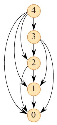
Figure 2: Subproblem graph for the rod cutting problem with (n=4) (Cormen et al. 2022).
Subproblem \(n=4\) is dependent on subproblems \(n=3\), \(n=2\), and \(n=1\). The bottom-up approach follows this dependency by ensuring that the subproblems are solved in the correct order.
Besides serving as a helpful visualization, depicting the problem using a DAG can also help to identify the time complexity of the problem. This is the sum of the time needed to solve each subproblem. Each problem of size \(n\) requires \(n-1\) subproblems to be solved, and each subproblem of size \(n-1\) requires \(n-2\) subproblems to be solved. This leads to a time complexity of \(O(n^2)\).
Reconstructing a Solution
The two dynamic programming solutions above return the maximum revenue that can be obtained by cutting up the rod. However, they do not return the actual cuts that should be made. This can be done by modifying the algorithms to store the cuts that are made. The code is given below.
def extended_bottom_up_cut_rod(p, n):
    r = [0 for _ in range(n+1)]
    s = [0 for _ in range(n+1)]
    for j in range(1, n+1):
        q = -float('inf')
        for i in range(1, j+1):
            if q < p[i] + r[j-i]:
                q = p[i] + r[j-i]
                s[j] = i
        r[j] = q
    return r, s

def print_cut_rod_solution(p, n):
    r, s = extended_bottom_up_cut_rod(p, n)
    while n > 0:
        print(s[n])
        n -= s[n]
In the bottom-up approach, the table s is used to store the size of the first piece to cut off. The function print_cut_rod_solution uses this table to print the cuts that should be made.
Matrix-chain Multiplication
The next problem covered by Cormen et al. is matrix-chain multiplication (Cormen et al. 2022). Given a sequence of matrices \(A_1, A_2, \ldots, A_n\), where the dimensions of matrix \(A_i\) are \(p_{i-1} \times p_i\), determine the most efficient way to multiply the matrices. The problem is to determine the order in which the matrices should be multiplied so that the number of scalar multiplications is minimized.
Understanding the solution to this problem requires understanding the problem itself. Depending on the order in which matrices are multiplied in a chain, the number of scalar multiplications can vary. Consider three matrices \(A \in \mathbb{R}^{10 \times 100}\), \(B \in \mathbb{R}^{100 \times 5}\), and \(C \in \mathbb{R}^{5 \times 50}\). The number of scalar multiplications required to compute \((AB)C\) is \(10 \times 100 \times 5 + 10 \times 5 \times 50 = 7500\), while the number of scalar multiplications required to compute \(A(BC)\) is \(10 \times 100 \times 50 + 100 \times 5 \times 50 = 75000\). The order in which the matrices are multiplied can have a significant impact on the number of scalar multiplications required.
Matrix multiplication is associative, so the order in which the matrices are grouped does not matter. The key to solving this problem is to find the most efficient way to group the matrices. The first part of the solution is to determine the number of possible groupings, or parenthesizations, we can make.
Determining Parenthesizations
The number of possible parenthesizations of a chain of \(n\) matrices is given by \(P(n)\). When \(n \geq 2\), the number of possible parenthesizations is given by
\[ P(n) = \sum_{k=1}^{n-1}P(k)P(n-k). \]
A brute force solution to this problem would require \(O(2^n)\) time (see Exercise 14.2-3 in (Cormen et al. 2022)).
Dynamic Programming Solution
We now review the four step process to formulating a dynamic programming solution as put forth by Cormen et al. (Cormen et al. 2022).
Optimal Substructure
What is the optimal substructure of this problem? Consider matrix-chain sequence \(A_{i:j} = A_i A_{i+1} \cdots A_j\). If we split the sequence at \(k\), then the optimal solution to the problem is the optimal solution to the subproblems \(A_{i:k}\) and \(A_{k+1:j}\). This is because the number of scalar multiplications required to compute \(A_{i:j}\) is the sum of the number of scalar multiplications required to compute \(A_{i:k}\) and \(A_{k+1:j}\) plus the number of scalar multiplications required to compute the product of the two subproblems.
How can we ensure that there is not a more optimal grouping of \(A_{h:l}\), where \(i \leq h < k\) and \(k < l \leq j\)? The answer lies in evaluating all possible splits.
Recursive Solution
What is the cost of an optimal solution to the problem? We must first compute the minimum cost of parenthesizing \(A_{i:j}\) for \(1 \leq i \leq j \leq n\). Let \(m[i,j]\) be the minimum number of scalar multiplications needed to compute \(A_{i:j}\). Starting with the base case, \(m[i,i]\) is the cost to compute the multiplication of a single matrix, which is 0. Assuming optimal subproblems are chosen, \(m[i,j] = m[i,k] + m[k+1,j] + p_{i-1}p_kp_j\), where the last term is the cost of multiplying \(A_{i:k}A_{k+1:j}\).
All possible splits must be evaluated. So, how many are there? Omitting the first and last matrices, there are \(j - i\) possible splits. We can now define the optimal solution in terms of the following recursion:
\[ m[i,j] = \min \{m[i,k] + m[k+1,j] + p_{i-1}p_kp_j : i \leq k < j\}. \]
Storing the Solutions
The problem is taking shape and we have a recursive formula. However, this is no better than the brute-force method until we figure out how to select the optimal subproblems and store their solutions. That is, we need to optimally select \(k\). A bottom-up approach involves computing the cost of all possible combinations of the \(n\) matrices and building up from there. This requires \(O(n^2)\) memory to store both the costs \(m[i, j]\) as well as the value of \(k\) that splits them \(s[i, j]\).
def matrix_chain_order(p):
    n = len(p) - 1
    m = [[0 for _ in range(n)] for _ in range(n)]
    s = [[0 for _ in range(n)] for _ in range(n)]
    for l in range(2, n+1):
        for i in range(1, n-l+2):
            j = i + l - 1
            m[i][j] = float('inf')
            for k in range(i, j):
                q = m[i][k] + m[k+1][j] + p[i-1]*p[k]*p[j]
                if q < m[i][j]:
                    m[i][j] = q
                    s[i][j] = k
    return m, s
The function matrix_chain_order computes the cost of all possible combinations of the \(n\) matrices and stores the value of \(k\) that splits them. The outer-most for loop controls the length of the chain being evaluated. We start at 2 since the cost of a length 1 chain is 0. Intuition tells us that the triply-nested for loop has a time complexity of \(O(n^3)\).
This algorithm computes the cost in ascending order of chain length. When \(l=2\), the cost of all chains of length 2 is computed. When \(l=3\), the cost of all chains of length 3 is computed, and so on. The recursion in the inner-most nested loop will only ever access the entries in m which have been previously computed.
Reconstructing a Solution
We now have a solution which generates the optimal number of scalar multiplications needed for all possible combinations of the \(n\) matrices. However, we do not yet have a solution which tells us the order in which the matrices should be multiplied. This information is held in s, which records the value of \(k\) that splits the chain. The function print_optimal_parens is given below.
def print_optimal_parens(s, i, j):
    if i == j:
        print(f"A_{i}", end="")
    else:
        print("(", end="")
        print_optimal_parens(s, i, s[i][j])
        print_optimal_parens(s, s[i][j]+1, j)
        print(")", end="")
Using figure 14.5 from (Cormen et al. 2022) as a reference, we can test the function print_optimal_parens. It is first called as print_optimal_parens(s, 1, 6). This recursively calls print_optimal_parens(s, 1, 3) and print_optimal_parens(s, 4, 6). We will work from left to right, top to bottom and fill out the values.
Second call: print_optimal_parens(s, 1, 3)
This recursively calls print_optimal_parens(s, 1, 1) and print_optimal_parens(s, 2, 3). We can see that this first call has \(i==j\), so it prints \(A_1\). The second call prints \((A_2A_3)\). This initial call already set up the first set of parenthesis, so the intermediate result is \(((A_1(A_2A_3))\cdots)\).
Third call: print_optimal_parens(s, 4, 6)
This recursively calls print_optimal_parens(s, 4, 5) and print_optimal_parens(s, 6, 6). This first call will recursively call print_optimal_parens(s, 4, 4) and print_optimal_parens(s, 5, 5). This produces \((A_4A_5)\) from the first subcall and \(A_6\) from the second subcall. The intermediate result is now \((\cdots((A_4A_5)A_6))\).
Putting it all together
Combining these results yields \(((A_1(A_2A_3))((A_4A_5)A_6))\). This is the optimal parenthesization of the matrix chain \(A_1A_2A_3A_4A_5A_6\).
Applying Dynamic Programming
Section 14.3 of (Cormen et al. 2022) focuses on the two core components of a dynamic programming solution: optimal substructure and overlapping subproblems. By taking a closer look at how these two components were used in various dynamic programming solutions, you should have a greater understanding of how to apply dynamic programming to new problems.
As shown in previous examples, determining the optimal substructure is the first step in formulating a dynamic programming solution. In most cases, this comes from understanding the problem itself well. It is the result of a natural way of analysis and decomposition of the problem. When learning a new concerto, a musician must have a strong command of technique and fundamental musical concepts. Similarly, a strong understanding of the problem is required to determine the optimal substructure.
Determining Optimal Substructure
- Show that a solution to a problem requires making a choice, like where to cut in the rod cutting problem.
- Assume that you are given an optimal choice.
- Identify the subproblems that result from this choice.
- Show that solutions to these subproblems are optimal.
In the last step, we are typically looking for a contradiction. The assumption of step 2 means that if we end up finding a more optimal solution to a subproblem, then the original choice was not optimal. The result is that we have a better overall solution.
The efficiency of a dynamic programming solution depends on the number of subproblems times the number of choices we have for each subproblem. When investigating solutions to a new problem, it is better to start with a simple case and expand outward as necessary. Using a subproblem graph is a great way to visualize the subproblems and their dependencies.
Counter-Example: The Longest Simple Path
Consider the following problems which first appear to have optimal substructure.
- Shortest path: find a path \(u \leadsto v\) with the fewest edges without cycles.
- Longest simple path: find a path \(u \leadsto v\) with the most edges without cycles.
The first problem has optimal substructure. Suppose that the shortest path \(u \leadsto v\) is given by \(p\). Given some intermediate vertex \(w\), the optimal path from \(u \leadsto w\) is given by \(p_1\) and the optimal path from \(w \leadsto v\) is given by \(p_2\). If there were a shorter path \(p’_1\) from \(u \leadsto w\) then we could replace \(p_1\) with it and get a total path with fewer edges.
Check your understanding
Why does that argument reinforce the idea of optimal substructure? By showing that the optimal solution to a subproblem is the optimal solution to the original problem. This argument becomes clearer as we consider the longest simple path problem.
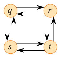
Figure 3: Subproblem graph for the longest simple path problem (Cormen et al. 2022).
Consider the directed graph above. The path \(q \rightarrow r \rightarrow t\) is the longest simple path from \(q\) to \(t\). Keep in mind that the problem is to find a simple path with the most edges. If the substructure is optimal, then the subpaths must also exhibit maximal edges. The subpath \(q \leadsto r\) in this case is simply \(q \rightarrow r\), but the longest simple path from \(q\) to \(r\) is \(q \rightarrow s \rightarrow t \rightarrow r\). Therefore, the subpath \(q \leadsto r\) is not optimal. This is a counter-example to the idea that the longest simple path problem has optimal substructure.
The longest simple path problem does not have independent subproblems. Consider a path from \(q\) to \(t\). This could be broken down into subproblem \(q \leadsto r\) and \(r \leadsto t\). For \(q \leadsto r\), we have \(q \rightarrow s \rightarrow t \rightarrow r\). This subproblem is dependent on \(s\) and \(t\), so we cannot use them in the second subproblem \(r \leadsto t\) without forming a path that is not simple. Specifically, the first subproblem includes \(t\), so the second subproblem cannot include \(t\). However, the second subproblem MUST include \(t\).
Questions
- What are the independent subproblems in the rod cutting and matrix-chain multiplication problems?
Using Overlapping Subproblems
First, do not confuse the idea of overlapping subproblems with the need for the subproblems to be independent. Subproblems are independent if they do not share resources, which the longest simple path problem does not have. Overlapping subproblems means that a subproblem may require the result of another independent subproblem. This is the case in the rod cutting problem, where the value of a subproblem is used in the calculation of the value of the next subproblem.
A desirable trait of any recursive problem is that it have a small number of unique subproblems. The running time of such a solution is dependent on the number of subproblems, so having more of them will naturally lead to a less efficient solution. Section 14.3 reviews the bottom-up solution to matrix-chain multiplication, specifically focusing on the number of times the solution of each subproblem is required. It is recommended to review this section for further understanding.
Questions
- How many subproblem solutions are reused in the rod cutting problem of \(n=4\)?
- How many subproblem solutions are reused when computing the Fibonacci sequence of \(n\)?
Longest Common Subsequence
A longest common subsequence (LCS) of two input sequences \(X = \langle x_1, x_2, \ldots, x_m \rangle\) and \(Y = \langle y_1, y_2, \ldots, y_n \rangle\) is a sequence \(Z = \langle z_1, z_2, \ldots, z_k \rangle\) such that \(Z\) is a subsequence of both \(X\) and \(Y\) and \(k\) is as large as possible. For example, given \(X = \langle A, B, C, B, D, A, B \rangle\) and \(Y = \langle B, D, C, A, B, A \rangle\), the LCS is \(\langle B, C, A, B \rangle\).
The subsequence is not necessarily consecutive! A subsequence \(Z\) is common to a sequence \(X\) if it corresponds to a strictly increasing sequence of indices such that \(x_{i_j} = z_j\).
Naive Solution
First, how would we solve this problem using a brute-force method? We could generate all possible subsequences of \(X\) and \(Y\) and then compare them. This would require \(O(n2^m)\) time.
Dynamic Programming Solution
Following the four step process, we can formulate a dynamic programming solution to the LCS problem. Step 1 is to determine the optimal substructure of the problem.
Optimal Substructure
Let \(X = \langle x_1, x_2, \ldots, x_m \rangle\) and \(Y = \langle y_1, y_2, \ldots, y_n \rangle\). Let \(Z = \langle z_1, z_2, \ldots, z_k \rangle\) be an LCS of \(X\) and \(Y\).
- If \(x_m = y_n\), then \(z_k = x_m = y_n\) and \(Z_{k-1}\) is an LCS of \(X_{m-1}\) and \(Y_{n-1}\).
- If \(x_m \neq y_n\) and \(z_k \neq x_m\), then \(Z\) is an LCS of \(X_{m-1}\) and \(Y\).
- If \(x_m \neq y_n\) and \(z_k \neq y_n\), then \(Z\) is an LCS of \(X\) and \(Y_{n-1}\).
The theorem above shows that the LCS problem has optimal substructure. Let’s break this down a bit. Consider two sequences (words): rocinante and canterbury. The longest common subsequence is “cante”. Since the last characters of the two original words do not match, we can remove the last character from either word and find the LCS of the two remaining words. This implies that we could have found the LCS of the two original words by finding the LCS of a smaller subproblem.
What if the two words had the same last character? The LCS of the shorter strings is the same as the LCS of the original strings with the last character removed.
Recursive Solution
The next step is to write a recursive solution to the problem. Given the substrucure just presented, a bottom-up approach seems intuitive. Starting with indices \(i=0\) and \(j=0\) which indicate the length of the current strings \(X_i\) and \(Y_j\), increase the length and compute the LCS as we go.
Define \(c[i, j]\) as the LCS length of \(X_i\) and \(Y_j\). The goal is to compute \(c[m,n]\), where \(m\) and \(n\) are the lengths of \(X\) and \(Y\), respectively. The recursive formula is given by
\[ c[i, j] = \begin{cases} 0 & \text{if } i = 0 \text{ or } j = 0, \\ c[i-1, j-1] + 1 & \text{if } i, j > 0 \text{ and } x_i = y_j, \\ \max(c[i-1, j], c[i, j-1]) & \text{if } i, j > 0 \text{ and } x_i \neq y_j. \end{cases} \]
-
Example: “atom” and “ant”
The LCS of “atom” and “ant” is “at”. The tree below shows the recursive calls to each subproblem. A dashed line indicates that the subproblem has already been solved.
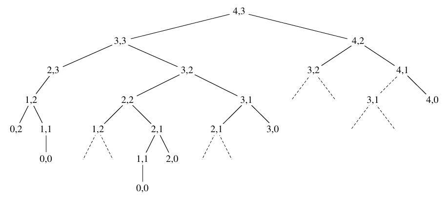
Figure 4: Recursion tree for the LCS problem (Cormen et al. 2022).
Storing the Solutions
The LCS problem has \(\Theta(mn)\) distinct subproblems, so storing the solutions to these subproblems will allow us to avoid redundant computation. A dynamic programming solution goes as follows:
- Store the lengths of the LCS of the prefixes of \(X\) and \(Y\) in a table \(c\).
- Additionally store the solution to the subproblems in a table \(b\) so that we can reconstruct the LCS.
- The entries are filled in a row-major order.
The code is given below.
def lcs_length(X, Y):
    m = len(X)
    n = len(Y)
    b = [[0 for _ in range(n+1)] for _ in range(m+1)]
    c = [[0 for _ in range(n+1)] for _ in range(m+1)]
    for i in range(1, m+1):
        for j in range(1, n+1):
            if X[i-1] == Y[j-1]:
                c[i][j] = c[i-1][j-1] + 1
                b[i][j] = "↖"
            elif c[i-1][j] >= c[i][j-1]:
                c[i][j] = c[i-1][j]
                b[i][j] = "↑"
            else:
                c[i][j] = c[i][j-1]
                b[i][j] = "←"
    return c, b

def print_lcs(b, X, i, j):
    if i == 0 or j == 0:
        return
    if b[i][j] == "↖":
        print_lcs(b, X, i-1, j-1)
        print(X[i-1], end="")
    elif b[i][j] == "↑":
        print_lcs(b, X, i-1, j)
    else:
        print_lcs(b, X, i, j-1)
Reconstructing a Solution
Printing the solution starts with the last entry in the table \(b\). If the entry is “↖”, then the last characters of \(X\) and \(Y\) are the same and we print the character. If the entry is “↑”, then we move up in the table. If the entry is “←”, then we move left in the table.
Exercises
- Exercise 14.1-5 from (Cormen et al. 2022).
- Exercise 14.2-1 from (Cormen et al. 2022).
- Write a recursive function to compute the Fibonacci sequence. What is the time complexity of this function? What is the time complexity of the dynamic programming solution?
- Write a function that prints a table similar to Figure 14.8 from (Cormen et al. 2022) for the LCS problem.