Edge Detection
Introduction
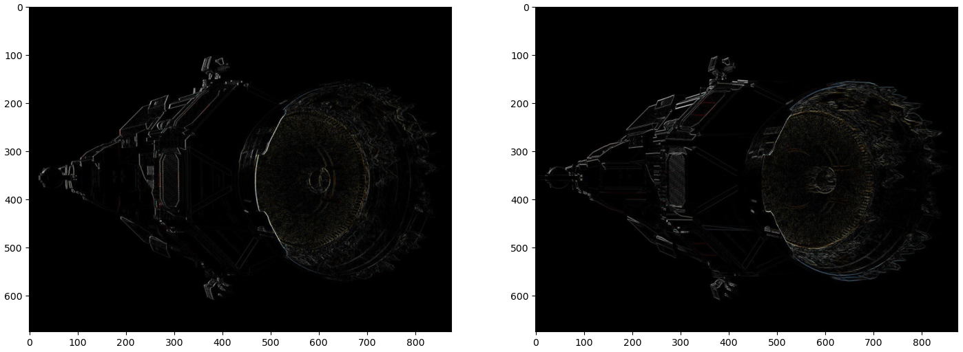
Figure 1: Vertical derivative filter (left) and horizontal derivative filter (right).
When image gradient filters are applied to an image, we can observe that the sample responses are very sensitive to noise and detail. For example, look at the surface at the back of ship near the drive cone. To resolve this, the image should be smoothed before differentiating it. Recall that the Gaussian filter smooths the area so that neighboring pixels are more similar than distant pixels.
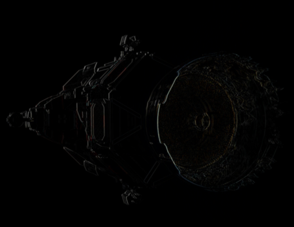
Figure 2: dx kernel applied to image blurred with Gaussian (sigma=1).
This is closer to what we want, but the end goal is to create an image that shows distinct edges. We need to be clear about what an edge is. For now, we consider the images produced by convolving the \(dx\) or \(dy\) kernels as edge score images. They are only intermediate; we still need to make a final decision.
In this section, we will learn about the Canny Edge Detector. The general algorithm is as follows:
- Smooth the image using Gaussian blurring.
- Compute the gradient image via filtering. Most commonly, the Sobel operator is used.
- Filter out weaker edge score by selecting local pixels with the largest gradient change.
- Use double thresholding to separate strong, or definite, edge pixels from weak ones.
- Remove all weak pixels not connected to a strong pixel.
Canny edge detection follows 3 objective criteria:
- Edges should be detected with a low error rate. The goal is to extract as many actual edges as possible.
- A detected edge should correspond to the center pixel of the edge in the original image.
- It should be robust to noise and only mark an edge pixel once.
Smoothing the image can be done by applying a Gaussian blur. Next, we need to compute the gradient image.
Computing Gradient Norms
As we saw before, the derivative filters compute the direction of greatest change in the calculated direction. When combining the result of \(dx\) and \(dy\), we get the gradient of the pixel.
\[ \nabla f(x, y) = \Bigg[\frac{\partial f}{\partial x}, \frac{\partial f}{\partial y}\Bigg]. \]
Canny edge detection works by selecting local pixels with the largest gradient change. In order to do this, we need to compute the norm of the gradient. If we consider every pixel in the gradient image to be a vector indicating the direction of greatest change, the norm can be computed as
\[ \|\nabla f(x, y)\| = \sqrt{\Big(\frac{\partial f}{\partial x}\Big)^2 + \Big(\frac{\partial f}{\partial y}\Big)^2}. \]
Additionally, we want the angle of direction of the gradient. This can be computed for each pixel as
\begin{equation*} \theta = \text{atan2}(\frac{\partial f}{\partial x}, \frac{\partial f}{\partial y}). \end{equation*}
In practice, this can be computed at the same time. There are also efficient implementations of atan2 which can generate an array of the same size of the original image containing the computed angles for each pixel.
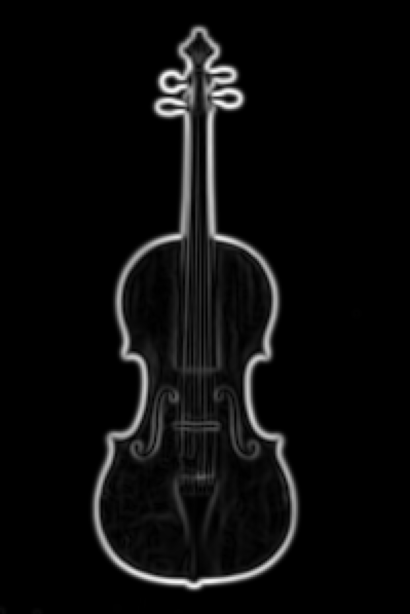
Figure 3: Gradient norm of image.
The figure above shows the result of computing the gradient norms for each pixel. This representation is intuitive to interpret. The largest values are on the edges of the violin. The image produced by this step is still too fuzzy. These do not represent the final edges.
Nonmaxima Suppression
The gradient norm image is helpful in showing all edge scores, but the egdes are still too thick and there are many disconnected edge scores detected. We can thin the edges by evaluating neighboring pixels. We will select only the local pixels which have the highest absolute gradient and suppress the others. This process is called nonmaxima suppression. There are two approaches to this problem. The first is approximates the closest gradient normal. The second uses interpolation to compute a more accurate value.
In the first approach, the number of discrete orientations for the edge normal are split into horizontal, vertical, \(45^{\circ}\), and \(-45^{\circ}\).
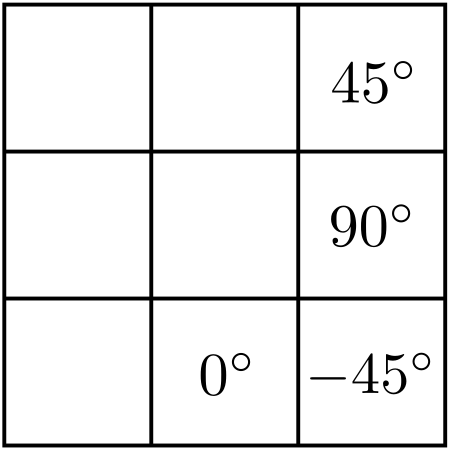
Figure 4: Discretizing angles into 4 regions.
For a given pixel, the gradient direction is discretized into one of the above four regions by selection the angle closest to the original angle given. Next, the gradient norm of the given pixel is compared to that of the pixels on either side of it following the same discretized direction. If one of the neighboring pixels has a higher gradient norm, the current pixel’s value is set to 0. The intuition here is that if it were an edge pixel, it would have the largest gradient norm along its given direction.
The result of applying this process on our gradient image is shown below.
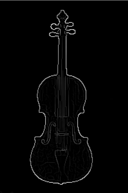
Figure 5: Gradient norm image after nonmaxima suppression is applied.
Interpolation
An alternative approach is to interpolate the gradient norm using the actual angle. Instead of discretizing it into one of four regions above, the original angle is used to compute the neighboring pixels in continuous space. This will, of course, produce invalid pixel locations. The gradient norm for the neighboring pixels follows the approach discussed in Sampling and Aliasing.
For example, if we are at pixel \((5, 5)\) with a gradient direction of \(55^{\circ}\), then the neighboring pixels along that angle can be computed by first finding the vector following that direction. That is
\begin{align*} \mathbf{p}_{\text{offset}} &= \begin{bmatrix} \cos (55^{\circ} \cdot \frac{\pi}{180^{\circ}})\\ \sin (55^{\circ} \cdot \frac{\pi}{180^{\circ}}) \end{bmatrix}\\ &= \begin{bmatrix} .5736\\ .8192 \end{bmatrix} \end{align*}
Then the two neighboring pixels along this direction are \(f(5 - .5373, 5 - .8192)\) and \(f(5 + .5373, 5 + .8192)\). These are clearly not valid pixel locations. To compute the interpolated value, a weighted contribution from the closest 4 pixels are used for each of the two neighbors. For \(f(4.4627, 4.1808)\), these pixels are \(\{(4, 4), (5, 4), (4, 5), (5, 5)\}\). The interpolation weights for this pixel are computed as
\begin{align*} w_x &= 4.4627 - 4 = .4627\\ w_y &= 4.1808 - 4 = .1808 \end{align*}
Then the resulting pixel value is computed via bilinear interpolation:
\begin{align*} f(4.4627, 4.1808) &= (1 - w_x) \cdot (1 - w_y) \cdot f(4, 4)\\ &+ w_x \cdot (1 - w_y) \cdot f(5, 4)\\ &+ (1 - w_x) \cdot w_y \cdot f(4, 5)\\ &+ w_x \cdot w_y \cdot f(5, 5). \end{align*}
Thresholding
We now have an image of edge scores, but have not yet made a final determination on which pixels are actually edges. One approach to selecting the edge pixel is to use thresholding. That is, we suppress any pixel value that is lower than some parameter \(T\):
\[ f_{T}(x, y) = f(x, y) \geq T. \]
However, this approach will still leave many false positives as well as edge segments that may be connected to strong edges. This issue is partly resolved via hysteresis thresholding. For this, we choose 2 threshold values: one for weak edges and another for strong edge scores. Using these scores, we can generate two images:
\begin{align*} f_{T_H}(x, y) &= f(x, y) \geq T_{H}\\ f_{T_L}(x, y) &= f(x, y) \geq T_{L} \end{align*}
We can then eliminate the duplicate pixels in \(f_{T_L}\) by subtracting \(f_{T_H}\):
\[ f_{T_L} = f_{T_L} - f_{T_H}. \]
Using the image processed via nonmaxima suppression from before, this generates the following images:
Figure 6: Low threshold image (left) and high threshold image (right).
Connectivity Analysis
There must be a reason why we computed a lower threshold. There are weak edge pixels that may have been apart of a segment connected to strong pixels. In this case, we want to keep every weak pixel that is 8-connected to a strong pixel.
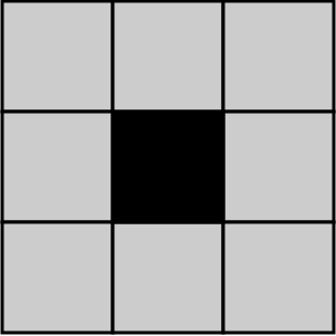
Figure 7: The pixels surrounding the black pixel are 8-connected to it. Source: Wikipedia
This can be accomplished with the following steps:
- Locate an edge pixel in the high threshold image.
- Mark all pixels in the weak image that are 8-connected to the current strong pixel as strong pixels.
- Repeat steps 1 and 2 for all strong pixels in the original high threshold image.
- Set all pixels in the weak image that were not marked to 0.
- Add the marked weak pixels to the strong image.
Applying the procedure above given the weak and strong images from before yields the following result.
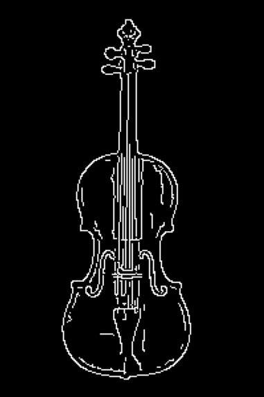
Figure 8: Final edge image after connectivity analysis.