GPU Pattern: Convolution
This pattern involves tiling and input data staging.
Recall from Lab 1 where we implementing a kernel to blur an image. This kernel worked on each individual output pixel by computing the weighted average of each pixel from the input image, centered on the output pixel location. When we implemented this, we set the weight of every pixel to 1. Whether you were aware of it or not, you implemented a convolution between an input image and weighted kernel.
The convolution is an extremely important operator that works on time-varying signals of different dimensionality. In computer vision, they are commonly used to compute responses between a known pattern and an input image. The pixels that return a greater response as a result of convolution indicate a match between the pattern and the input image.
This operator can and has been efficiently implemented in a GPU. Through studying this pattern, you will learn to utilize constant memory storage and shared memory storage to efficiently implement a convolution kernel. These techniques will be useful in later applications as well.
Convolution
A convolution is a function that takes two functions as input and produces a third function as output. The first function is the input and the second function is the kernel. The output is called the feature map. The kernel is also sometimes called the filter.
\[ (f * g)(t) = \int f(t-a)g(a)da \]
We can view them more concretely by considering the functions to be vectors. For example, let the function \(f\) be an input vector \(x\) and \(w\) be a kernel representing a filter. The convolution operator is then
\[ (x * w)(t) = \int x(t-a)w(a)da. \]
The result the feature map representing the response of the kernel at each location in the input.
In the case of discrete values, it is common to use an odd-sized kernel and center it on an input value. The kernel size is given by some radius \(r\). The convolution operator is then
\[ (x * w)(t) = \sum_{-r}^r x(t-r)w( r). \]
The figure below shows an example of a 1D convolution of a vector if size 8 with a kernel of size 5, centered on the \(t = 2\).
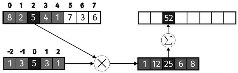
Figure 1: 1D Convolution between a vector of size 8 and a kernel of size 5.
Convolution is defined in such a way that the kernel is traversed in an inverted manner. In the example above, \(y_2\) is computed by applying the kernel to \(\mathbf{x}\) centered on \(x_2\). The calculation in terms of the locations accesses is
\[ y_2 = x_4 w_{-2} + x_3 w_{-1} + x_2 w_0 + x_1 w_1 + x_0 w_2. \]
This operation is very similar to the correlation operator, which is defined as
\[ (x \star w)(t) = \sum_{-r}^r x(t+r)w( r). \]
We can use the correlation operator to compute the convolution by flipping the kernel. In this case, the calculation can be represented using the dot product. We can also slightly adjust the indexing so that the first index is 0.
\[ y_i = \sum_{k=0}^{2r} x_{i+k-r} w_{2r-k}. \]
Note that the convolution shown above would be undefined for \(i = 0\) and \(i = 1\) since the kernel would be accessing negative indices. Based on the definition, we would ignore these values. This is called a valid convolution. The output size is then \(n - 2r\). There is also a full convolution where the output size is \(n\). In this case, the kernel is padded with zeros so that it can be applied to all elements of the input.
2D Convolution
Image convolutions use 2D filters applied to 2D images. For a filter with radius \(r\), size of the filter is \((2r + 1) \times (2r + 1)\). The convolution is then
\[ (x * w)(i, j) = \sum_{-r}^r \sum_{-r}^r x(i-r, j-r)w(r, s). \]
Properties of Convolutions
Convolutional networks are commonly built on full or valid convolutions. Other variants have also been explored. Here, we will briefly discuss the different properties of this operator. A more detailed treatment can be found in (Dumoulin and Visin 2018).
Padding
By definition, a convolution of an input with a filter of size \(n\times n\) will produce an output of size \((m-n+1)\times(m-n+1)\), where \(m\) is the size of the input. This means that the output will be smaller than the input. This is often referred to as a valid convolution. The figure below shows a convolution between a \(3\times3\) kernel and a \(5\times5\) input.
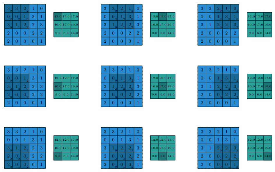
Figure 2: A valid convolution (Dumoulin and Visin 2018).
The output of this convolution is a \(3\times3\) feature map. This is a problem if we want to build a deep network. Each convolution will reduce the size of the input. If we were to stack multiple convolutional layers, the output would eventually be too small to be useful. If we want our output to be same size as the input, we can add padding to the original input image before convolving it. This is often known as a full convolution. An example is shown below.
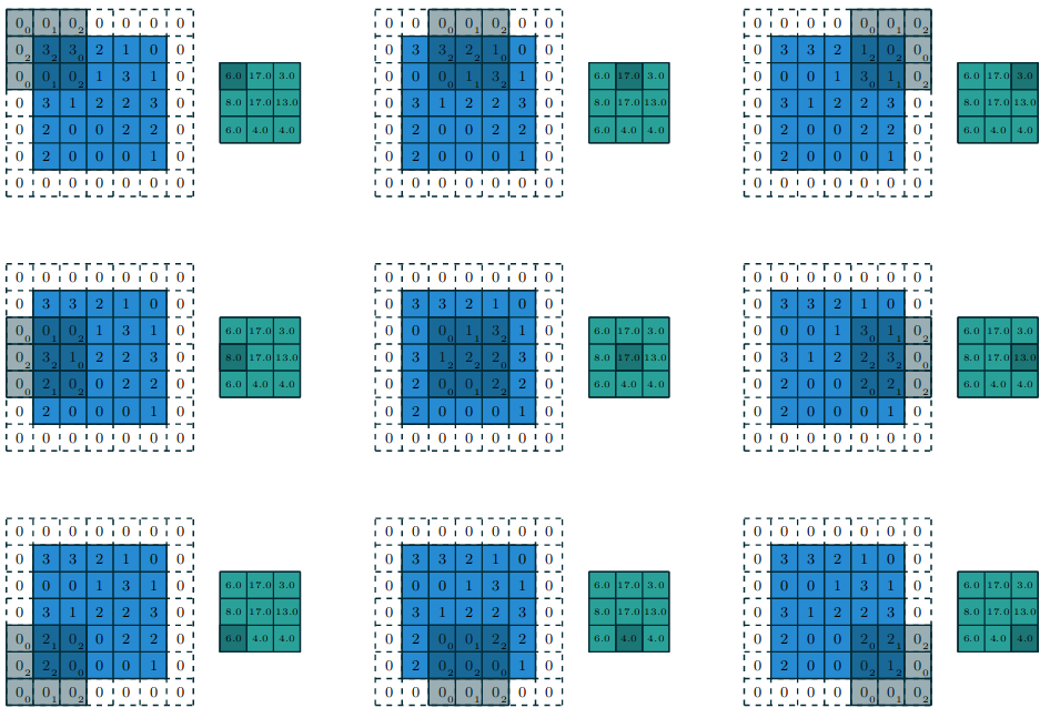
Figure 3: A full convolution (Dumoulin and Visin 2018).
Stride
So far, we have only looked at convolutions which step by 1 unit as they shift over the image. We can control the size of this step, or stride, to produce different outcomes. Picking a non-unit stride has a number of effects on the features that are learned in a convolutional neural network.
- Dimensionality reduction: Skipping over pixels reduces the size of the output feature map. This provides another way of downsampling the input.
- Less computation: Fewer computations are required to produce the output feature map.
- Increased field of view: A larger stride increases the field of view of the kernel, leading to larger receptive fields in deeper layers.
Given an input of size \(m\times m\) and a kernel of size \(n\times n\), the output size of a convolution with stride \(s\) is given by
\[ \left\lfloor\frac{m-n}{s}\right\rfloor + 1. \]
The figure below shows a convolution with stride 2 on a \(5\times5\) input.
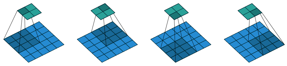
Figure 4: A convolution with stride 2 (Dumoulin and Visin 2018).
Kernel Size
The size of the kernel has a large impact on the features that are learned. A larger kernel will have a larger receptive field. This means that the kernel will be able to capture more information about the input. However, this comes at the cost of increased computation. Common kernel sizes in most CNNs are \(3\times3\), \(5\times5\), and \(7\times7\). It is also convenient to pick an odd kernel size so that the kernel has a center pixel.
Dilation
Around 2015, a research trend for CNNs was to find a way to increase the receptive field without adding more parameters. The result is a dilated convolution. The output of a dilated convolution is computed by skipping over pixels in the input. The figure below shows a \(3\times3\) kernel with a dilation of 2.
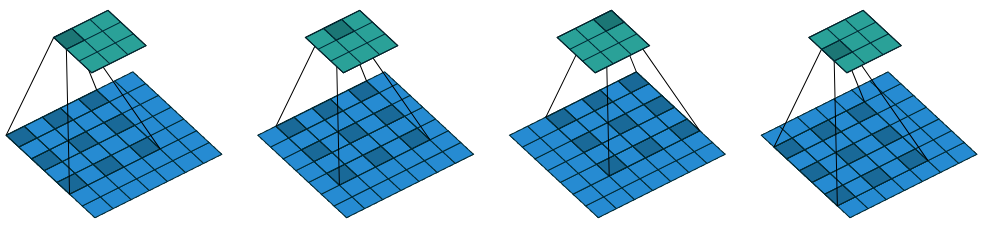
Figure 5: A dilated convolution (Dumoulin and Visin 2018).
The output size is computed as
\[ \left\lfloor\frac{m + 2p - n - (n-1)(d-1)}{s}\right\rfloor + 1, \]
where \(p\) is the amount of padding and \(d\) is the dilation factor.
Implementing a Convolution Kernel
It is straightforward to write the convolution operation in CUDA C++. Each thread will compute the value for a single output pixel using the filter. We already implemented something very similar with the blurring kernel. The kernel itself should accept the following arguments:
- The input image
- The output image
- The kernel
- The radius of the kernel
- The width of the output image
- The height of the output image
A more robust implementation would consider things like padding, stride, dilation, and whether or not a valid or full convolution is desired. For now, we will focus on the simplest case: a valid convolution with a stride of 1 and no padding or dilation. First, let’s review the initial naive solution from Programming Massively Parallel Processors (Hwu, Kirk, and El Hajj 2022).
__global__ void conv2D(float *input, float *filter, float *output,
                       int r, int width, int height) {
    int outCol = blockIdx.x * blockDim.x + threadIdx.x;
    int outRow = blockIdx.y * blockDim.y + threadIdx.y;

    float sum = 0.0f;
    for (int row = 0; row < 2*r+1; row++) {
        for (int col = 0; col < 2*r+1; col++) {
            int inRow = outRow + row - r;
            int inCol = outCol + col - r;
            if (inRow >= 0 && inRow < height && inCol >= 0 && inCol < width) {
                sum += input[inRow * width + inCol] * filter[row * (2*r+1) + col];
            }
        }
    }
    output[outRow * width + outCol] = sum;
}
With this kernel, the input and output sizes are assumed to be the same. There is a boundary check in the inner-most loop to account for pixels for which a convolution cannot be computed. Based on this check, we can see that this kernel is performing a valid convolution. The extra \(2r\) pixels on each side of the output are skipped. This presents a computational problem in the form of control divergence. Recall that all threads in a warp must execute the same instruction. If the boundary check fails for some threads, they will still execute the instructions in the loop, but will not contribute to the output. This is a waste of resources.
It is also a waste of resources in terms of memory used for the output. If we already know that we want to perform a valid convolution, we can allocate the output image to be the appropriate size before calling it. A slightly modified version is shown below.
__global__ void conv2D(float *input, float *filter, float *output,
                       int r, int width, int height) {
    int outCol = blockIdx.x * blockDim.x + threadIdx.x;
    int outRow = blockIdx.y * blockDim.y + threadIdx.y;

    float sum = 0.0f;
    for (int row = 0; row < 2*r+1; row++) {
        for (int col = 0; col < 2*r+1; col++) {
            int inRow = outRow + row;
            int inCol = outCol + col;
            sum += input[inRow * width + inCol] * filter[row * (2*r+1) + col];
        }
    }
    output[outRow * width + outCol] = sum;
}
Constant Memory and Caching
There is a much larger issue present in both versions of this kernel in terms of memory bandwidth. Similar to the matrix multiplication kernel, this kernel can benefit from tiling. However, there is a new problem that arises specifically with convolution. The same filter is accessed by every single thread. This filter does not change for the entire duration of the kernel. This means that we are wasting memory bandwidth by having every thread access the same filter.
Given its relatively small size, this kernel is a perfect candidate for constant memory. This is a special type of memory that is cached on the GPU. It is read-only and has a limited size, but it is much faster than global memory. We can write to the devices constant memory from the host code.
#define FILTER_RADIUS 1
__constant__ float kFilter_d[2*FILTER_RADIUS+1][2*FILTER_RADIUS+1];
This informs the compiler to allocate a 2D array of floats in constant memory. The size of the array is determined by the constant `FILTER_RADIUS`. We can then copy the filter to the device using the `cudaMemcpyToSymbol` function.
cudaMemcpyToSymbol(kFilter_d, filter_h, (2*FILTER_RADIUS+1)*(2*FILTER_RADIUS+1)*sizeof(float));
The line above assumes there is some data on the host in the array `filter_h`. This array is copied to the device. A small note on naming convention, Google’s C++ style guide recommends naming constant variables with a k prefix. I have adopted this convention here.
At this point, kFilter_d is accessible from the kernel as a global variable. There is no need to pass it as an argument. The kernel can be modified to use this constant memory as follows.
__global__ void conv2D(float *input, float *output,
                       int r, int width, int height) {
    int outCol = blockIdx.x * blockDim.x + threadIdx.x;
    int outRow = blockIdx.y * blockDim.y + threadIdx.y;

    float sum = 0.0f;
    for (int row = 0; row < 2*r+1; row++) {
        for (int col = 0; col < 2*r+1; col++) {
            int inRow = outRow + row;
            int inCol = outCol + col;
            sum += input[inRow * width + inCol] * F_d[row][col];
        }
    }
    output[outRow * width + outCol] = sum;
}
If you organize your files such that the kernel is in a separate file from the host code, you will need to declare the constant variable in the kernel file as well.
Constant memory variables are stored in DRAM with global memory. The CUDA runtime will cache them since it knows they will not be modified. Processors use caches to reduce the latency of memory accesses by keeping frequently used data in a small, fast memory that is often located directly on the chip. This type of constant cache is preferable to one that would support high-throughput writes in terms of chip design. It would require specialized hardware to support both which would increase the cost of the chip.
Tiled Convolutions
Even with caching, the convolutional kernel still makes many accesses to DRAM. Similar to matrix multiplication, we can tile the input image to reduce the number of accesses. Similar to that example, we will use a \(4 \times 4\) tile size. If the input is a \(16 \times 16\) image and we apply a kernel with radius \(r=2\), the output image under a valid convolution will be \(12 \times 12\). This is visualized in the figure below.
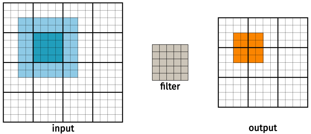
Figure 6: Left: The input image and its tiling. Middle: the filter. Right: The output image and its tiling.
The parallel solution to this problem will follow the tiled approach used for matrix multiplication. One key difference in this case is that the input tile size will be larger than the output tile size. This size difference would further be complicated if we left the kernel size as a parameter.
Following the design presented by (Hwu, Kirk, and El Hajj 2022) in Chapter 7, there are two immediate approaches to this problem based on the tile size. The first is to choose a block size that matches the size of the input tiles. The benefit to this approach is that each thread can load a single input element into shared memory. The drawback is that some of the threads will be disabled when computing the output value since the output tile is smaller. This is a form of control divergence and will result in wasted resources.
#define FILTER_RADIUS 1
#define IN_TILE_DIM 4
#define OUT_TILE_DIM ((IN_TILE_DIM) - 2*(FILTER_RADIUS))
__constant__ float kFilter_d[2*FILTER_RADIUS+1][2*FILTER_RADIUS+1];
__global__ void conv2DTiledConstKernel(float *input, float *output,
                                       int width, int height) {
    __shared__ float inputTile[IN_TILE_DIM][IN_TILE_DIM];
    // Input tile coordinates
    int col = blockIdx.x * OUT_TILE_DIM + threadIdx.x;
    int row = blockIdx.y * OUT_TILE_DIM + threadIdx.y;
    if (row < height && col < width) {
        inputTile[threadIdx.y][threadIdx.x] = input[row * width + col];
    } else {
        inputTile[threadIdx.y][threadIdx.x] = 0.0f;
    }
    __syncthreads();

    // Output tile coordinates
    int tileCol = threadIdx.x - FILTER_RADIUS;
    int tileRow = threadIdx.y - FILTER_RADIUS;

    // In a valid convolution, the output is smaller than the input
    row -= FILTER_RADIUS;
    col -= FILTER_RADIUS;

    if (tileCol >= 0 && tileCol < OUT_TILE_DIM && tileRow >= 0 && tileRow < OUT_TILE_DIM) {
        float sum = 0.0f;
        for (int fRow = 0; fRow < 2*FILTER_RADIUS+1; fRow++) {
            for (int fCol = 0; fCol < 2*FILTER_RADIUS+1; fCol++) {
                sum += inputTile[tileRow + fRow][tileCol + fCol] * kFilter_d[fRow][fCol];
            }
        }
        output[row * (width - 2 * FILTER_RADIUS) + col] = sum;
    }
}
There are a few things to consider here. The first phase of this kernel collaboratively loads data into a shared memory space, similar to what we have seen before. This kernel assumes a convenient indexing scheme where the row and column will always be >= 0. We could adopt a scheme that centers the convolution on the center point of the kernel by allowing for negative indices. In this case, it would be necessary to check if the row and column are less than 0. This implementation only needs to verify that the row and column are within the given image size.
When it comes to computing the output, not every thread will contribute. This is depicted by the lightly shaded areas in the figure below. You should also note which threads are active for output computation per block. In this simple example, a \(3 \times 3\) filter is used. The input tile dimension is \(4 \times 4\) which means the output tile will be \(2 \times 2\). Only the threads corresponding to the darker blue on the left contribute to the output calculation. Since this one block computes 4 output values, the next block should start 2 units to the right of this one.
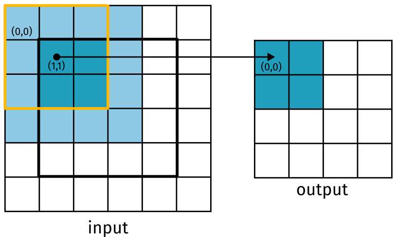
Figure 7: The active threads for computing the output tile.
Performance Analysis
The purpose of this approach was to increase the ratio of arithmetic operations to global memory accesses. For the threads that compute an output tile, there is one multiplication and one addition which yields \(\mathtt{OUT\_TILE\_DIM}^2*(2*\mathtt{FILTER\_RADIUS} + 1)^2*2\) operations total. Each thread in the input tile loads a single float value for a total of \(\mathtt{IN\_TILE\_DIM}^2 * 4\) bytes. For our small example above, this gives
\[ \frac{2^2 * 3^2 * 2}{4^2 * 4} = 1.125\ \text{Ops/byte}. \]
In a more realistic example, we would maximize our input tile size to take advantage of the available threads on the device. Currently, the maximum number of supported threads is 1024. This allows for an input tile size of \(32 \times 32\). The resulting operations per byte under this tile size is
\[ \frac{30^2 * 3^2 * 2}{32^2 * 4} = 3.955\ \text{Ops/byte}. \]
This ratio increases with the size of the filter.
Caching the Halo Cells
In the previous example, the size of the input tile compared to the output tile means that there were some threads that did not contribute to the output computation. These are the threads managing the lightly shaded cells in the figure above. We will refer to these as halo cells.
This implementation is going to take advantage of the caching behavior in the chip itself. Values that have been recently used are more likely to already be in L2 cache. This is a safe assumption since the neighboring blocks will have loaded these values into shared memory. This means that the input and output tile sizes can be the same; there is no need to waste any threads in the block. The full kernel is given below.
__global__ void conv2DTiledCachedConstKernel(float *input, float *output,
                                             int width, int height) {
    __shared__ float inputTile[IN_TILE_DIM][IN_TILE_DIM];
    // Input tile coordinates
    int col = blockIdx.x * IN_TILE_DIM + threadIdx.x;
    int row = blockIdx.y * IN_TILE_DIM + threadIdx.y;
    if (row < height && col < width) {
        inputTile[threadIdx.y][threadIdx.x] = input[row * width + col];
    } else {
        inputTile[threadIdx.y][threadIdx.x] = 0.0f;
    }
    __syncthreads();

    if (row < FILTER_RADIUS || col < FILTER_RADIUS || col >= (width - FILTER_RADIUS) || row >= (height - FILTER_RADIUS)) return;

    // Output tile coordinates
    row -= FILTER_RADIUS;
    col -= FILTER_RADIUS;
    int tileCol = threadIdx.x - FILTER_RADIUS;
    int tileRow = threadIdx.y - FILTER_RADIUS;

    float sum = 0.0f;
    for (int fRow = 0; fRow < 2 * FILTER_RADIUS + 1; fRow++) {
        for (int fCol = 0; fCol < 2 * FILTER_RADIUS + 1; fCol++) {
            // If this value is in shared memory, access it there
            if (tileCol + fCol >= 0 &&
                tileCol + fCol < IN_TILE_DIM &&
                tileRow + fRow >= 0 &&
                tileRow + fRow < IN_TILE_DIM) {
                sum += inputTile[tileRow + fRow][tileCol + fCol] * kFilter_d[fRow][fCol];
            } else {
                // Otherwise, access it from global memory
                sum += input[(row + fRow) * width + (col + fCol)] * kFilter_d[fRow][fCol];
            }
        }
    }

    output[row * (width - 2 * FILTER_RADIUS) + col] = sum;
}