GPU Pattern: Parallel Scan
What is it?
- Parallelizes sequential problems.
- Works with computations that can be described in terms of a recursion.
- Used as a primitive operation for sorting, tree operations, and recurrences.
- Studying this will also reveal how parallelization can increase the complexity beyond that of a traditional sequential approach.
Example: Inclusive Scan
Given an array of numbers, the inclusive scan computes the sum of all elements up to a given index. For example, given the array [1, 2, 3, 4, 5], the inclusive scan would produce [1, 3, 6, 10, 15]. You could solve this recursively, but it would be horribly inefficient. A sequential solution is achievable with dynamic programming. However, a parallel solution is much more efficient.
void sequential_scan(float *x, float *y, uint N) {
    y[0] = x[0];
    for (uint i = 1; i < N; i++) {
        y[i] = y[i - 1] + x[i];
    }
}
Naive Parallel Reduction
If we have \(n\) elements, we could have \(n\) threads each compute the sum of a single element. How many operations would that take? The first thread computes the sum of 1 element, or 0 operations. The second thread computes the sum of 2 elements, 1 operation, and so on. This can be described as a sum of the first \(n\) natural numbers, which is \(n(n + 1)/2\). This parallel solution is worse than the sequential solution, coming in at \(O(n^2)\).
Kogge-Stone Algorithm
The first solution to this problem relies on GPU Pattern: Reduction and is called the Kogge-Stone algorithm. The algorithm was published in 1973 by Peter M. Kogge and Harold S. Stone during their time at Stanford University.
Adapting the Reduction Tree
Design reduction tree so that each thread has access to relevant inputs. The input matrix is modified to that input \(A_i\) contains the sum of up to \(2^k\) elements after \(k\) iterations. For example, after iteration 2, \(A_3\) contains the sum \(A_0 + A_1 + A_2 + A_3\).
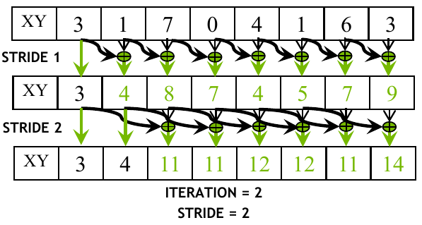
Figure 1: Visualization of parallel inclusive scan based on the Kogge-Stone algorithm (Source: NVIDIA DLI).
This is implemented in the following code:
__global__ void Kogge_Stone_scan_kernel(float *X, float *Y, unsigned int N) {
        __shared__ float A[SECTION_SIZE];
        unsigned int i = blockIdx.x * blockDim.x + threadIdx.x;

        if (i < N) {
            A[threadIdx.x] = X[i];
        } else {
            A[threadIdx.x] = 0;
        }

        for (unsigned int stride = 1; stride < blockDim.x; stride *= 2) {
            __syncthreads();
            float temp;
            if (threadIdx.x >= stride) {
                temp = A[threadIdx.x] + A[threadIdx.x - stride];
            }
            __syncthreads();
            if (threadIdx.x >= stride) {
                A[threadIdx.x] = temp;
            }
        }

        if (i < N) {
            Y[i] = A[threadIdx.x];
        }
}
It is not possible to guarantee that a block can cover the entire input, so SECTION_SIZE is used to ensure that the input is covered. This should be the same as the block size. Each thread starts off by loading its initial input into shared memory. Starting with thread 2, each thread computes a sum of the value assigned to its thread as well as the one before it by a factor of stride.
The loop itself is moving down the reduction tree, which is bounded logarithmically. The local variable temp is used to store the intermediate result before barrier synchronization takes place. Otherwise there would be a possibility of a write-after-read race condition.
Double Buffering
The temporary variable and second call to __syncthreads() are necessary since a thread may read from a location that another thread is writing to. If the input and output arrays were represented by two different areas of shared memory, this call could be removed. This approach is called double-buffering.
It works as follows: the input array is read from global memory into shared memory. At each iteration the data read from the first array is used to write new values to the second array. Since the values used in that iteration are only read from the first array, the second array can be used as the input array for the next iteration. This cycle continues back and forth until the final result is written to the output array.
Efficiency Analysis
Work efficiency is a measure of how efficient a particular algorithm is compared to the minimum number of operations required. For inclusive scan, the minimum number of add operations required is \(n - 1\), yielding an efficiency of \(O(n)\). During each iteration of the Kogge-Stone algorithm, each thread iterates over a loop that is logarithmic in size. That is, it starts with a stride of 2, then 4, 8, \(\dots \frac{n}{2}\). This yields a complexity of \(O(n \log_2 n)\).
Due to the parallel nature of the algorithm, it still requires fewer steps than the sequential algorithm. The details muddy the water a bit as threads that stop execution early still expend resources from the device. In general, we can say that the parallel algorithm takes \(\frac{1}{m} n \log_2 n\) steps, where \(m\) is the number of execution units. If we have as many execution units as we have elements, then we only need \(\log_2 n\) steps.
Brent-Kung Algorithm
Sharing intermediate results Distribute to different threads Reduction tree Sub-sums used to calculate some of the scan output values Brent-Kung follows the same idea as Kogge-Stone, but with better work efficiency.
Use reduction tree on the first \(n/2\) elements, then use the results to reverse the tree.
At the start of the reverse direction, the elements with index \(2^i - 1\), for \(i = 1, 2, \dots, \log_2 n\), already have the correct value.
Figure 2: Visualization of parallel inclusive scan based on the Brent-Kung algorithm (Source: NVIDIA DLI).
The figure above shows the state of the algorithm before the reverse direction begins. The second half is better seen as a table of values. The row labeled Initial contains the state of the array after the first half of the algorithm is completed. For the values that already have their correct value, no update is needed. The two rows following Initial show the state of the array after the first and second iterations of the reverse direction.
| 0 | 1 | 2 | 3 | 4 | 5 | 6 | 7 | |
|---|---|---|---|---|---|---|---|---|
| Initial | 0 | 0…1 | 2 | 0…3 | 4 | 4…5 | 6 | 0…7 |
| Iteration 1 | 0…5 | |||||||
| Iteration 2 | 0…2 | 0…4 | 0…6 |
Implementing the Forward Half
The relevant reduction tree phase of Brent-Kung is implemented in CUDA C++ below.
for (uint stride = 1; stride <= blockDim.x; stride *= 2) {
    __syncthreads();
    if ((threadIdx.x + 1) % (stride * 2) == 0) {
        A[threadIdx.x] += A[threadIdx.x - stride];
    }
}
From the perspective of threadIdx.x = 7, the first iteration would add the value from threadIdx.x = 6 to its own value. On the next iteration, the stride offset would add threadIdx.x = 5. Thread 5 already has the sum from 4 and 5 before being added to 7, so 7 now has the sums from indices 4 through 7. On its last iteration, the value for stride is now 4, and 7 adds the value from 3 to its own value. This is the final result for the first half of the algorithm.
There is a lot of control divergence present in this code. Since fewer threads stay active as the loop goes on, it is better to organize the threads such that they are contiguous. We can do that with slightly more complicated indexing, so that contiguous threads use data from the active portions of the array.
for (uint stride = 1; stride <= blockDim.x; stride *= 2) {
    __syncthreads();
    int index = (threadIdx.x + 1) * 2 * stride - 1;
    if (index < blockDim.x) {
        A[index] += A[index - stride];
    }
}
Thread 0 maps to index, thread 1 maps to index 3, thread 2 to index 5, and so on. Only when the number of active threads drops below the warp size does control divergence become a problem.
Implementing the Reverse Half
The reverse half of the algorithm is implemented in CUDA C++ below.
for (uint stride = blockDim.x / 4; stride > 0; stride /= 2) {
    __syncthreads();
    int index = (threadIdx.x + 1) * 2 * stride - 1;
    if (index + stride < blockDim.x) {
        A[index + stride] += A[index];
    }
}
Continuing the example from above, the first thread threadIdx.x = 0 maps to index 3. This will load the value from index 3 and add it to the value at index 5. At that point, the value at index 5 will be the sum of the values from indices 0 through 5.
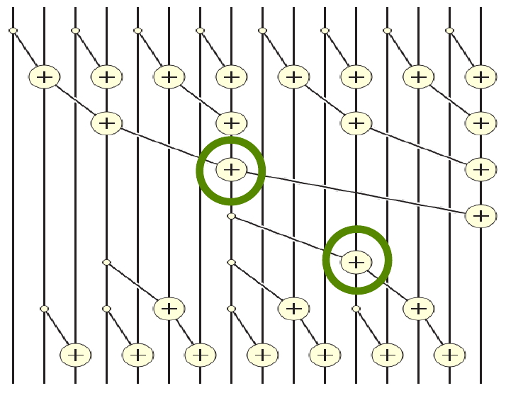
Figure 3: Full Brent-Kung visualization (source: NVIDIA DLI).
Efficiency Analysis
The reduction tree of the first half of the algorithm require \(n - 1\) operations. For \(n\) elements, the reverse half requires \((2 - 1) + (4 - 1) + \dots + (n/2 - 1)\) operations for a total of \(N - 1 - \log_2 n\). This yields a work efficiency of \(O(n)\). Even though the theoretical work efficiency is better than Kogge-Stone, doesn’t mean its performance will always be better in practice. The drop off in active threads for Brent-Kung is much more severe than Kogge-Stone. It also requires additional steps to perform the reverse half. In general, Kogge-Stone is a better choice when we have more execution units, owing to its better parallelism.
The full code is given below.
__global__ void Brent_Kung_scan_kernel(float *X, float *Y, uint N) {
    __shared__ float A[SECTION_SIZE];
    unsigned int i = 2 * blockIdx.x * blockDim.x + threadIdx.x;

    if (i < N) {
        A[threadIdx.x] = X[i];
    }
    if (i + blockDim.x < N) {
        A[threadIdx.x + blockDim.x] = X[i + blockDim.x];
    }

    for (uint stride = 1; stride <= blockDim.x; stride *= 2) {
        __syncthreads();
        int index = (threadIdx.x + 1) * 2 * stride - 1;
        if (index < blockDim.x) {
            A[index] += A[index - stride];
        }
    }

    for (uint stride = blockDim.x / 4; stride > 0; stride /= 2) {
        __syncthreads();
        int index = (threadIdx.x + 1) * 2 * stride - 1;
        if (index + stride < blockDim.x) {
            A[index + stride] += A[index];
        }
    }
    __syncthreads();

    if (i < N) {
        Y[i] = A[threadIdx.x];
    }
    if (i + blockDim.x < N) {
        Y[i + blockDim.x] = A[threadIdx.x + blockDim.x];
    }
}
Adding Coarsening
Similar to other problems such as tiled matrix multiplication, if the hardware does not meet the capacity ti parallelize the entire problem, the price for parallelization is wasted. In such cases, we can coarsen the problem so that the available resources are fully utilized. Each thread will execute a phase of sequential scan, which is more work efficiency than other of the solutions presented above.
Phase 1
Such a solution starts off by performing a sequential scan. The threads can also collaborate in the beginning to load data into shared memory.
Phase 2
In the next phase, the threads execute a parallel scan via Kogge-Stone or Brent-Kung. Since each thread has already performed a sequential scan. This phase starts off with the last element assigned to each thread.
Phase 3
In the last phase, each thread adds its last value to the first \(n-1\) elements of the next section, where \(n\) is the number of elements assigned to each thread.
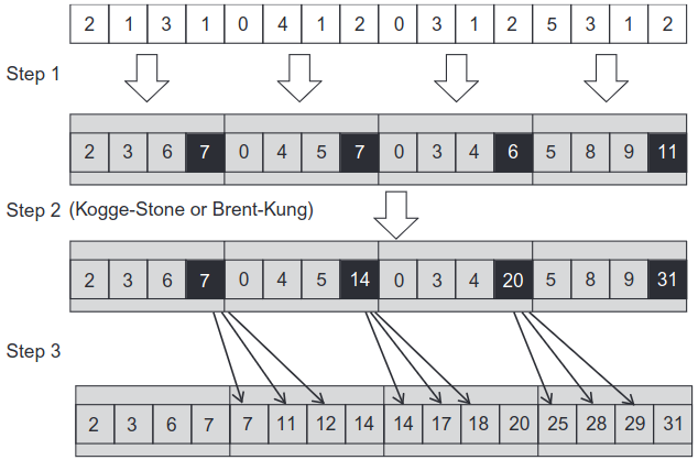
Figure 4: Three-phase parallel scan (Hwu, Kirk, and El Hajj 2022).
Segmented Parallel Scan
Input to scan operations may be too large to fit in memory. Hierarchical scans can be used to solve this problem. Partition input so that each section fits into shared memory for an SM. Another kernel launches after this is done to consolidate the results by adding the sum of the preceding scan blocks to each element of a scan block.
Each scan block is treated as an individual application of one of the previous kernels. Each successive scan block initially does not contain the sums of the preceding blocks. Those will be added in a separate kernel.
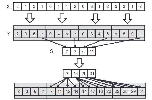
Figure 5: Segmented scan (Hwu, Kirk, and El Hajj 2022).
After each scan block has computed the scan for its partition, the last elements are then processed in the next step. However, these elements are all from different blocks, which means we must write them to a global space so they can all be accessed. Completing this step yields an array that has the final values of the scan corresponding to the indices from the original scan blocks (see the figure above). These values can then be used to update the preceding elements in each scan block to complete the scan.
Kernel 1: Section Scan
The first kernel essentially implements one of the previously discussed parallel scan kernels. The only difference is that the accumulation array is passed so that the blocks can write their output element values.
__syncthreads();
if (threadIdx.x == blockDim.x - 1) {
    accumulation[blockIdx.x] = A[threadIdx.x];
}
Kernel 2: Update Scan
For step 2, we need to run a parallel scan kernel like Kogge-Stone or Brent-Kung on the accumulation array.
Kernel 3: Update Elements
The final kernel takes the accumulated values and updates the original array so that all the elements have their correct scan value.
uint i = blockIdx.x * blockDim.x + threadIdx.x;
output[i] += accumulation[blockIdx.x - 1];
Optimizing Memory Efficiency
The previous solution provides a way of working with large inputs, but it is not memory efficient because of the need to store the accumulation array. There have been several attempts at optimizing this flow of information in the form of a stream-based scan. To understand the general strategy behind this approach, consider the segmented scan from the previous section.
The process starts by executing all the scan blocks in parallel. The first scan block has all the information it needs to compute the full scan for its partition. However, the second block needs the final output value from the first before it can update its own values. It will have to wait until block 0 has finished and written its value to global memory. It can then add that value to its own elements before sending its final value to the next block. This process continues until all the blocks have been processed.
To be clear, the first phase runs completely in parallel, and the second phase is sequential. If the final values are passed quickly enough between each block, the overall scan will still be efficient. Once each block has that passed value, it can continue its work in parallel since it is no longer dependent on the previous block.
For this to work, there needs to be a form of synchronization between blocks. The CUDA API does not provide grid-wide synchronization, so how can we accomplish this? One solution is to use a lock to effectively halt a thread until the value is ready to be read (Yan, Long, and Zhang 2013). The code below shows how this can be implemented.
__shared__ float previous_sum;
if (threadIdx.x == 0) {
    // Wait for previous flag
    while(atomicAdd(&flags[bid], 0) == 0);
    // Read previous partial sum
    previous_sum = scan_value[bid];
    // Propagate partial sum
    scan_value[bid + 1] = previous_sum + local_sum;
    // Memory fence
    __threadfence();
    // Update flag
    atomicAdd(&flags[bid + 1], 1);
}
__syncthreads();
The section ensures that only the first element of each block will perform this update. The flags array is a global array that is used to store the lock values. Once the flag is set to 1, the value from the global array scan_value is read and used to update the local sum. We haven’t used __threadfence() before, but it is used to ensure that the update to scan_value[bid + 1] is written before the call to atomicAdd is made.
Your first thought might be that there are too many global memory accesses. Shouldn’t this incur a large access penalty? Remember that many of these are overlapping values that were accessed by previous blocks, so they are most likely in the cache. Of course, if there is ever any doubt on the performance of a kernel, we can always profile it to verify our assumptions.
As opposed to the previous solution, this one only requires a single kernel. In the three kernel approach, there is no overlap between the values since each kernel is executed sequentially.
Preventing Deadlocks
This issue isn’t production ready just yet. Depending on how the blocks are scheduled, it is possible that a deadlock could occur. For example, the second block could be scheduled before the first block. If there aren’t enough SMs on the device then the first block will never be able to write its value to the global array. One solution to this is dynamic block index assignment.
In this approach, the block index assignment is not dependent on blockIdx.x. Instead it is assigned dynamically as blocks are processed.
__shared__ uint bid_s;
if (threadIdx.x == 0) {
    bid_s = atomicAdd(&block_index, 1);
}
__syncthreads();
uint bid = bid_s;
This ensures that each block gets a unique index and that the blocks are processed in the order they are ready.
The Takeaway
Parallel scan is a powerful tool for solving problems that can be described in terms of a recursion. The Kogge-Stone and Brent-Kung algorithms are two ways of parallelizing the scan operation. This problem presents a unique look at how tradeoffs must be made when parallelizing a problem. At the end of the day, we must work within the constraints of the hardware and framework made available to us.