GPU Performance Basics
Click here for slides accompanying these lecture notes.
These notes are on “Chapter 6: Performance Considerations” from the book Programming Massively Parallel Processors (Hwu, Kirk, and El Hajj 2022).
Memory Coalescing
Global memory accesses are one of the largest bottlenecks in GPU applications. DRAM has high latency based on its design. Each cell has a transistor and a capacitor. If the capacitor is charged, it represents a 1. The process to detect the charges in these cells is on the order of 10s of nanoseconds. DRAM can read consecutive groups of cells via bursts. This means that if the data we wish to access is stored consecutively, it can be accessed within the same burst. Contrast that was random access, in which the DRAM will have to make multiple bursts to read the required data. Memory coalescing refers to optimizing our global memory accesses to take advantage of DRAM bursts.
Matrices are naturally coalesced, so we have already been utilizing this performance pattern in previous examples.
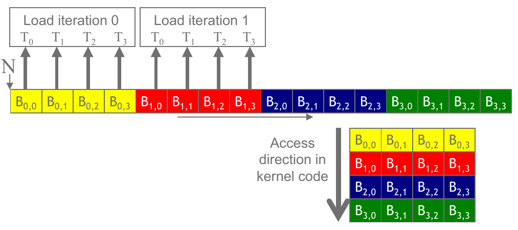
Figure 1: Memory accesses for a matrix in row-major ordering (Hwu, Kirk, and El Hajj 2022).
Strategies to optimize code for memory coalescing are to rearrange the threads, the data, or transfer the data first to shared memory so that accesses are faster, referred to as corner turning.
Example: Matrix Multiplication
Consider \(C = AB\), where \(A\) is in row-major order and \(B\) is in column-major order. The naive implementation of this algorithm will have poor memory coalescing. The figure below demonstrates the memory accesses for this scenario. The values required are not consecutive in memory, so the DRAM will have to make multiple bursts to read the data.
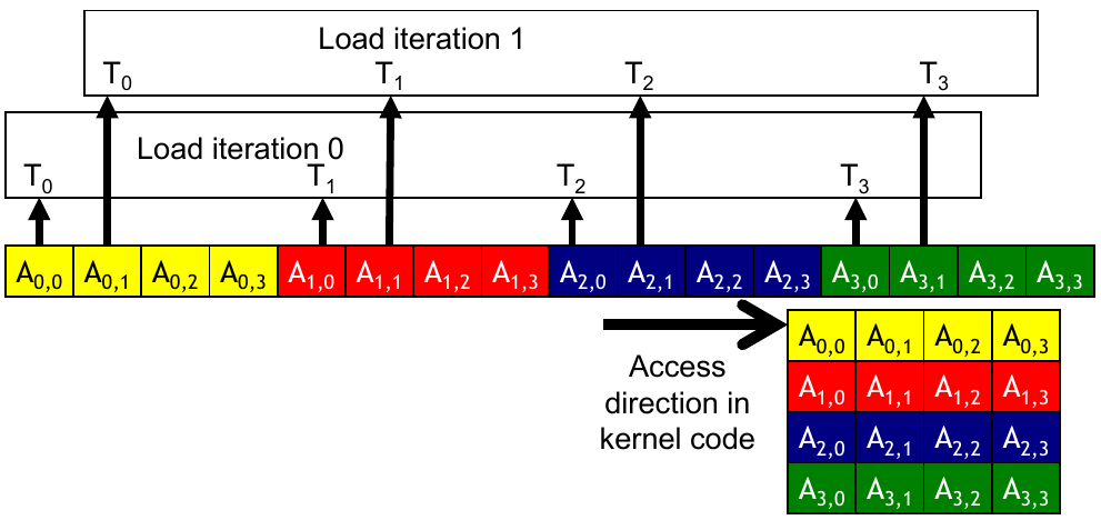
Figure 2: Memory accesses for a matrix in column-major ordering (Hwu, Kirk, and El Hajj 2022).
The accesses to the elements in \(B\) will be slower since the data is not coalesced. Accessing the elements is efficient if we assign \(N\) consecutive threads to load \(N\) consecutive elements from the same column of \(B\). This works in conjunction with tiling. The original loads to shared memory pull from consecutive elements in \(B\) which allows the application to take advantage of DRAM bursts. Once the data is in shared memory, the rest of the algorithm can be performed with coalesced accesses. Shared memory uses SRAM instead of DRAM, so coalescing is not an issue.
Hiding Memory Latency
DRAMS have banks and channels. A controller has a bus that connects banks to the processor. When the DRAM accesses data, the decoder enables the cells so that they can share the information stored with the sensing amplifier. This presents a high latency relative to the time it takes to actually transfer the data. This is why there are multiple banks per channel. The controller can initiate accesses on other banks instead of sitting and waiting for a single bank to finish.
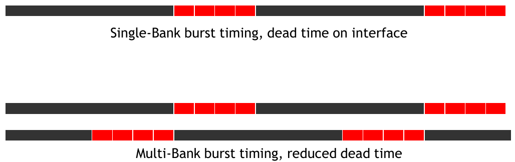
Figure 3: Single versus Multi-bank burst timings (Hwu, Kirk, and El Hajj 2022).
It is possible that the controller will initiate a request to a bank that is already busy. This is called a bank conflict. The controller will have to wait for the bank to finish its current request before it can service the new request. The more banks that are available, the less likely it is that a bank conflict will occur.
In CUDA, memory is coalesced at the warp level as 32-byte memory transactions. The warp controller can see the addresses requested by the warp and maps them into the 32-byte transaction (NVIDIA Blog).
Example: Matrix Multiplication
Consider DRAM with 4 channels and 2 banks per channel. The burst size of this DRAM is 8 bytes, or 2 elements. When data is written to DRAM in the first place, it is distributed in an interleaved fashion across the different channels and banks. The first figure below shows the input matrix \(M\) and output matrix \(P\). The second input matrix is omitted for brevity. The indices of \(M\) are linearized in row-major order to show how they are distributed across the DRAM banks. \(P\) is split into 4 blocks of size \(2 \times 2\).
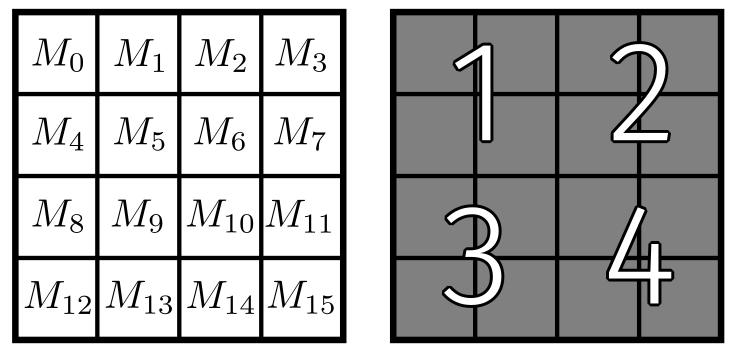
Figure 4: Matrix M with linearized indices and matrix P split into 4 blocks.
\(M\) is loaded into DRAM in an interleaved fashion. The first 8 bytes are loaded into bank 0 of channel 0. The next 8 bytes go into bank 0 of channel 1, and so on. Each burst returns 8 bytes. While the first access is being performed on bank 0 channel 0, the controller can initiate a request to bank 0 channel 1. This is visualized in the figure below.
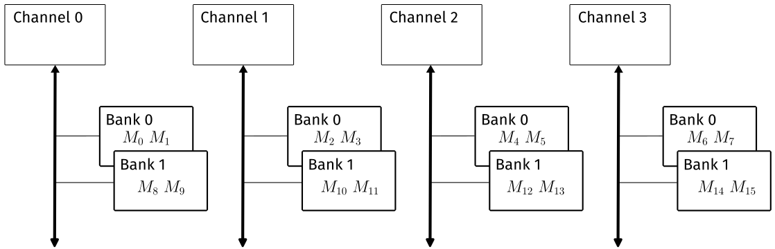
Figure 5: DRAM distribution for matrix M.
Given the distribution visualized above, we can see that the data accesses for the blocks of \(P\) will be coalesced. Output tile 1 in matrix \(P\) requires $M_0, M_1, M_4,$ and \(M_5\). The first two are available in a single burst from channel 0 bank 0, and the second two are available in a single burst from channel 2 bank 0.
Thread Coarsening
The price of parallelism may refer to the cost of
- launching threads
- synchronization
- redundant work
- redundant memory accesses
- etc.
It there are enough hardware resources available, parallelism at the finest level is ideal. If there are not enough resources, there is a price to pay for this parallelism. The hardware will need to serialize the work into blocks of threads that can be executed in parallel.
If this is the case for a particular application, it may be beneficial to apply some form of thread coarsening. If the hardware would serialize the work due to inefficient resources, the price of parallelism was paid for nothing. As the programmer, you have the ability to coarsen the threads to alleviate the price of parallelism.
Example: Coarsening Tiled Matrix Multiplication
In tiled matrix multiplication, it is possible that two separate blocks work with the same tile of data from an input matrix. We pay a price for this redundancy, but the benefit is that we can parallelize the work. If the hardware does not have sufficient resource, it will serialize these two blocks. This results in paying the price of data redundancy without the benefit of parallelism.
Let \(A, B \in \mathbb{R}^{6 \times 6}\), then \(C = AB \in \mathbb{R}^{6 \times 6}\). If we use a \(2 \times 2\) tile size, then we have 9 blocks of work that can be executed concurrently. For argument’s sake, let’s say that the hardware can only execute 3 blocks of work at a time. We can use thread coarsening to reduce the number of blocks to 3. Each block will be responsible for a single row of the tiled output matrix. That is, if the output matrix is \(6 \times 6\), then each block will be responsible for a \(2 \times 6\) tile of the output matrix. This is visualized in the figure below.
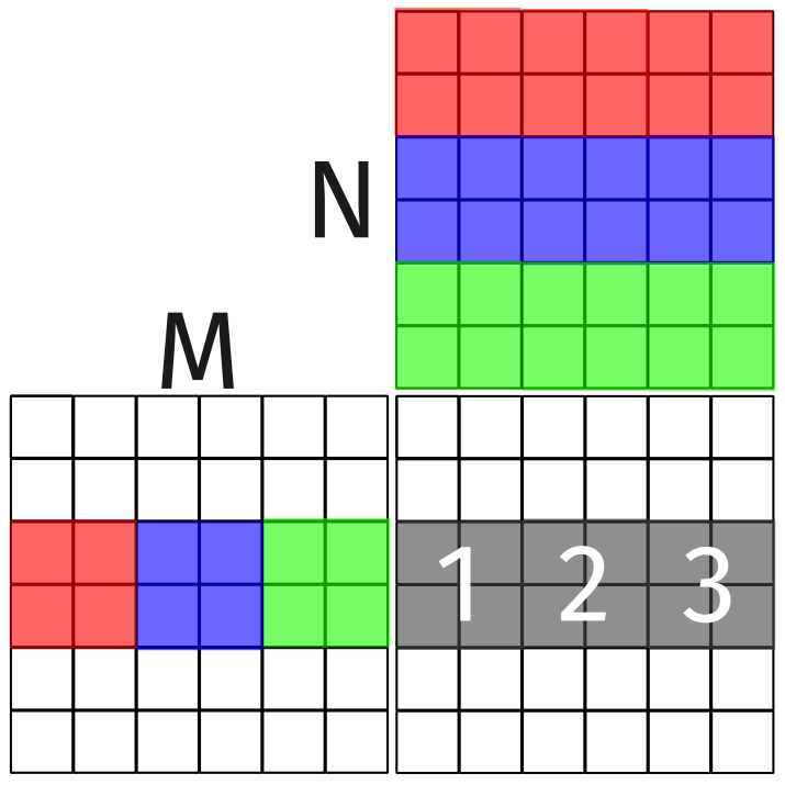
Figure 6: Thread coarsening for tiled matrix multiplication.
The block itself will perform a similar function as the implementation of tiled matrix multiplication we saw previously. We will need to modify the kernel so that it processes values to fill for 3 blocks of work, spanning each row. In the figure above, this is represented by the three gray, numbered blocks. Although each block uses a different column from matrix \(N\), they all use the same row from matrix \(M\). Our solution will take advantage of this reuse of data.
Consider the thread that computes the value for the top left entry of block 1. This thread will compute the output value as normal before looping to compute the corresponding relative position in blocks 2 and 3. That is, if the first entry computed is \((0, 0)\) of block 1, then the next entry computed will be \((0, 0)\) of block 2, and so on. This is visualized by the three solid black cells in the figure below.
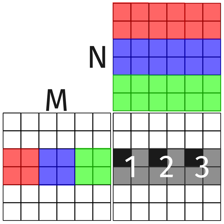
Figure 7: A single thread loops through three blocks as a result of thread coarsening.
The kernel code is given below. The additional loop controls the switch between the three consecutive tiles. The values from matrix M are loaded inside the outer-most loop and are reused across the coarse tiles.
#define TILE_WIDTH 2
#define COARSE_FACTOR 3
__global__ void matMulCoarse(float *M, float *N, float *P, int width) {
    __shared__ float Mds[TILE_WIDTH][TILE_WIDTH];
    __shared__ float Nds[TILE_WIDTH][TILE_WIDTH];

    int bx = blockIdx.x;
    int by = blockIdx.y;
    int tx = threadIdx.x;
    int ty = threadIdx.y;

    // Identify the row and column of the element to work on
    int row = by * TILE_WIDTH + ty;
    int colStart = bx * TILE_WIDTH * COARSE_FACTOR;

    // Initialize Pvalue
    float Pvalue[COARSE_FACTOR];
    for (int i = 0; i < COARSE_FACTOR; i++) {
        Pvalue[i] = 0.0f;
    }

    // Loop over the tiles required to compute the current output value
    for (int ph = 0; ph < width / TILE_WIDTH; ph++) {
        Mds[ty][tx] = M[row * width + ph * TILE_WIDTH + tx];

        for (int c = 0; c < COARSE_FACTOR; c++) {
            int col = colStart + c * TILE_WIDTH;

            Nds[ty][tx] = N[(ph * TILE_WIDTH + ty) * width + col];
            __syncthreads();

            for (int k = 0; k < TILE_WIDTH; k++) {
                Pvalue[c] += Mds[ty][k] * Nds[k][tx];
            }
            __syncthreads();
        }
    }

    for (int c = 0; c < COARSE_FACTOR; c++) {
        int col = colStart + c * TILE_WIDTH;
        P[row * width + col] = Pvalue[c];
    }
}
How to use coarsening in your applications
Thread coarsening is yet another technique that can be applied to optimize your parallel programs. The previous section demonstrated how it can be applied, but you are probably wondering when it should be applied. Deciding on whether to apply this technique is largely determined by careful analysis of your current application. This analysis should include benchmarking and profiling. There is work that provides an automatic solution (Stawinoga and Field 2018), but we will rely on determining that for ourselves.
For now, we can at least discuss when not to apply coarsening. The most obvious instance is when coarsening is completely unnecessary. Consider the vector addition kernel. Each thread performs an independent computation that has no overlapping data with other thread. There is no need to apply coarsening in this case.
Another bad case for implementation would be when the coarsening factor causes hardware to be underutilized. Parallelization in hardware is scalable. If we take away the opporunity for scale, there may be unused compute. This is typically something we can determine via benchmarking.
In the coarsened version of matrix multiplication above, we had to create additional private variables to store the coarsened values. These use additional registers per thread. If our application required more than the 32 registers available on our H100, for example, this would have a direct effect on occupancy. Keep that in mind when developing your thread coarsened solution.
Optimization Checklist
Section 6.4 of Programming Massively Parallel Processors (Hwu, Kirk, and El Hajj 2022) provides a checklist of items to consider when optimizing your GPU applications. These are summarized below.
Maximizing Occupancy
Having more threads than physical cores available is beneficial, as it hides the latency required for other operations such as data fetching. Instead of waiting on some operation to return, the hardware can switch to another thread to perform work. This is implemented by adjusting the launch configurations or optimizing the number of registers used per thread, for example. We also discussed solutions for hiding memory-based latency.
Coalesced Global Memory Accesses
Random accesses to memory are less efficient than consecutive ones. This is a theme that is repeated through many themes of computer science, such as sorting. Understanding of how the underlying hardware works brought to light new ways to optimize our applications. We can rearrange our data to take advantage of DRAM bursts, or we can use shared memory to reduce the latency of memory accesses.
Minimizing Control Divergence
Although we have not used any applications that exhibit control divergence, we have studied the concept. During SIMD execution, the hardware executes the same instructions on multiple data elements. If a thread or group of threads would diverge from the others, the hardware would have to make multiple passes to cover all of the possible paths.
Tiling
Global memory accesses exhibit higher latency due to the nature of DRAM. We can reduce the number of global memory accesses by using shared memory. This was exemplified in the tiled matrix multiplication examples, where there are many redundant data accesses. Moving these data to shared memory reduces the number of global memory accesses.
Thread Coarsening
In cases where the hardware would serialize execution of a kernel, thread coarsening can eliminate redundant work. In the tiled matrix multiplication example, we saw that the hardware would serialize execution of the kernel if there were not enough resources available. In this case, the same redundant loads to shared memory would be performed. To reduce this overhead, we coarsened the thread by having a single kernel perform the work of multiple blocks.
Identifying Bottlenecks
Knowing when to apply each of these optimization techniques comes down to understanding your application. The single most important step in optimizing your application is to identify the bottleneck. What resource is limiting the performance of your solution? Benchmarking and profiling are two techniques that can be used to identify these bottlenecks. We will begin learning these tools in the next lecture.
The Takeaway
At this point, you have learned the basics of GPU programming with CUDA. You should be familiar with writing kernels, setting launch configurations, and compiling them. You should be familiar with a few optimization techniques that can be applied to your applications, but you are probably not confident in your ability to identify when they should be used.
The next module of this course will focus on problems for which a straightforward solution is not obvious. These are problems that come from other domains of computer science, such as graph theory and linear algebra. We will learn how to apply the techniques we have learned to these problems, and we will learn new techniques that are specific to these problems. Even though the applications themselves may be specific, the techniques used to optimize them are not.