Gradient Boosting
Notes from (Friedman 2001)
-
Many machine learning methods are parameterized functions that are optimized using some numerical optimization techniques, notably steepest-descent.
-
Initial learner is a stump, subsequent learners are trees with depth as some power of 2 (commonly).
-
Numerical optimization in function space \[ g_m(\mathbf{x}) = E_y\Big[\frac{\partial L(y, F(\mathbf{x}))}{\partial F(\mathbf{x})}|\mathbf{x}\Big]_{F(\mathbf{x})=F_{m-1}(\mathbf{x})} \] The optimal step size found by solving
\[ \rho_m = \mathop{\arg \min}_{\rho} E_{y,\mathbf{x}}L(y,F_{m-1}(\mathbf{x})-\rho g_m(\mathbf{x})) \] Then the function \(m\) is updated: \[ f_m(\mathbf{x}) = -\rho_m g_m(\mathbf{x}) \]
Walking through it…
-
Make an initial guess with \(f_0(\mathbf{x})\)
-
Evaluate \(L(y, f_0(\mathbf{x}))\)
-
Improve model by boosting \(f_1(\mathbf{x}) = -\rho_1 g_1(\mathbf{x})\), where \[ g_1(\mathbf{x}) = \frac{\partial L(y, f_0(\mathbf{x}))}{\partial f_0(\mathbf{x})}. \] This implies that \(f_1\) is predicting the gradient of the previous function.
-
-
If the model is nonparametric, the expected value of the function conditioned on the input cannot be estimated accurately because we cannot sample the entire distribution of \(\mathbf{x}\). The author’s note that “…even if it could, one would like to estimate \(F^*(\mathbf{x})\) at \(\mathbf{x}\) values other than the training sample points.”
-
Smoothness is imposed by approximating the function with a parametric model. I think this means that the distribution is approximated as well.
\begin{equation} (\beta_m, \mathbf{a}_m) = \mathop{\arg \min}_{\beta, \mathbf{a}}\sum_{i=1}^N L(y_i, F_{m-1}(\mathbf{x}_i) + \beta h(\mathbf{x}_i; \mathbf{a})) \end{equation}
-
What if a solution to the above equation is difficult to obtain? Instead, view \(\beta_m h(\mathbf{x};\mathbf{a}_m)\) as the best greedy step toward \(F^*(\mathbf{x})\), under the constraint that the step direction, in this case \(h(\mathbf{x};\mathbf{a}_m)\), is a member of the class of functions \(h(\mathbf{x};\mathbf{a})\). The negative gradient can be evaluated at each data point: \[ -g_m(\mathbf{x}_i) = -\frac{\partial L(y_i, F_{m-1}(\mathbf{x}_i))}{\partial F_{m-1}(\mathbf{x}_i)}. \]
-
This gradient is evaluated at every data point. However, we cannot generalize to new values not in our dataset. The proposed solution comes via \(\mathbf{h}_m = \{h(\mathbf{x}_i;\mathbf{a}_m)\}_{1}^N\) “most parallel to” \(-\mathbf{g}_m \in \mathbb{R}^N\).
-
As long as we can compute a derivative for the original loss function, our subsequent boosting problems are solved via least-squared error: \[ \mathbf{a}_m = \mathop{\arg \min}_{\mathbf{a}, \beta} \sum_{i=1}^N \Big(-g_m(\mathbf{x}_i)-\beta h(\mathbf{x}_i;\mathbf{a})\Big)^2 \]
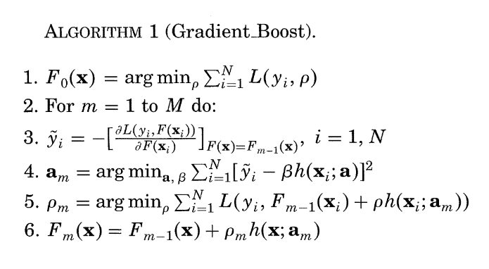
Figure 1: Original generic algorithm from (Friedman 2001).
Check out a basic implementation in Python here.
-