Greedy Algorithms
The slides for these notes can be found here.
Greedy algorithms are a class of algorithms that yield locally optimal solutions. In cases where the local optimum is also the global optimum, greedy algorithms are ideal. Even in cases where the global solution is more elusive, a local solution may be sufficient.
Activity Selection
Given a set of activities that need to be scheduled using a common resource, the activity selection problem is to find the maximum number of activities that can be scheduled without overlapping.
Each activity has a start time \(s_i\) and finish time \(f_i\), where \(0 \leq s_i < f_i < \infty\). An activity \(a_i\) takes place over the interval \([s_i, f_i)\). Two activities \(a_i\) and \(a_j\) are mutually compatible if \(s_i \geq f_j\) or \(s_j \geq f_i\).
Sort activities by their finish time. Objective: Find the largest subset of mutually compatible activities.
| \(i\) | 1 | 2 | 3 | 4 | 5 | 6 | 7 | 8 | 9 |
|---|---|---|---|---|---|---|---|---|---|
| \(s_i\) | 1 | 2 | 4 | 1 | 5 | 8 | 9 | 11 | 13 |
| \(f_i\) | 3 | 5 | 7 | 8 | 9 | 10 | 11 | 14 | 16 |
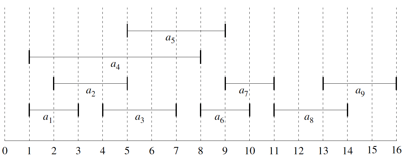
Figure 1: Visualization of activities over time (Cormen et al. 2022).
How many mutually compatible sets are there?
- \(\{a_1, a_3, a_6, a_8\}\)
- \(\{a_1, a_3, a_6, a_9\}\)
- \(\{a_1, a_3, a_7, a_9\}\)
- \(\{a_1, a_5, a_7, a_8\}\)
- \(\{a_1, a_5, a_7, a_9\}\)
- \(\{a_2, a_5, a_7, a_8\}\)
- \(\{a_2, a_5, a_7, a_8\}\)
Optimal Substructure
How do we verify that this problem has optimal substructure? First, it is important to formalize the problem based on the definition given previously. Define \(S_{ij}\) as the set of all activities that start after \(a_i\) finishes and finish before \(a_j\) starts.
\[ S_{ij} = \{a_k \in S : f_i \leq s_k < f_k \leq s_j\} \]
This defines a clear subset of the original set of data. That is, we have defined a subproblem of the original problem.
Which activities are those in \(S_{ij}\) compatible with?
- any \(a_i\) that finish by \(f_i\)
- any \(a_i\) that start no earlier than \(s_j\).
Given this subset, our subproblem is that of finding a maximum set of mutually compatible activities in \(S_{ij}\), denoted \(A_{ij}\). If \(a_k \in A_{ij}\), we are left with two subproblems:
- Find mutually compatible activities in \(S_{ik}\) – starts after \(a_i\) finishes and finish before \(a_k\) starts.
- Find mutually compatible activities in \(S_{kj}\) – starts after \(a_k\) finishes and finish before \(a_j\) start.
The two subsets above are defined as \(A_{ik} = A_{ij} \cap S_{ik}\) and \(A_{kj} = A_{ij} \cap S_{kj}\), respectively. Then \(A_{ij} = A_{ik} \cup \{a_k\} \cup A_{kj}\). The size of the set is given by \(|A_{ij}| = |A_{ik}| + 1 + |A_{kj}|\).
Claim: If our problem has optimal substructure, then the optimal solution \(A_{ij}\) must include optimal solutions for \(S_{ik}\) and \(S_{kj}\).
This claim can be proven using the cut-and-paste method used in Dynamic Programming. This technique works by showing that if a solution to a problem is not optimal, then there exists a way to cut the suboptimal portion and paste an optimal one. This will lead to a contradiction because the original was assumed to be optimal.
Proof: Suppose that \(A_{kj}\) is not optimal, and we could find a set \(A’_{kj}\) that is larger. Then we could replace \(A_{kj}\) with \(A’_{kj}\) in \(A_{ij}\) to obtain a larger set. This contradicts the assumption that \(A_{ij}\) is optimal.
Simply put, if the claim is that the given solution is optimal, and the solution is constructed from optimal solutions to subproblems, then there cannot exist any other solution that is better. Another way to look at this: if we construct optimal solutions to subproblems, then the solution to the original problem must be optimal.
Recursive Solution
Let \(c[i, j]\) be the size of the optimal solution for \(S_{ij}\). Based on the above discussion, the size is computed as
\[ c[i, j] = c[i, k] + c[k, j] + 1. \]
This dynamic programming solution assumes we know the optimal solution for all subproblems. To know this, we need to examine all possibilities which include \(a_k\) in the solution.
\[ c[i, j] = \begin{cases} 0 & \text{if } S_{ij} = \emptyset, \\ \max \{c[i, k] + c[k, j] + 1 : a_k \in S_{ij}\} & \text{if } S_{ij} \neq \emptyset. \end{cases} \]
Greedy Solution
The greedy solution is the naive one: select an activity that leaves the resource available for as many other activities as possible, which is the activity that finishes first. If multiple activities finish at the same time, select one arbitrarily.
The subproblem is that of finding a maximum size set of mutually compatible activities that start after \(a_1\) finishes. More generally, the optimal solution consists of all \(a_i\) that start after \(a_k\) finishes, where \(a_k\) is the last activity to finish:
\[ S_{k} = \{a_i \in S : s_i \geq f_k\}. \]
Is the greedy solution optimal? Suppose that \(a_m \in S_k\) is the activity that finishes first. Then it must be included in the maximum size subset of mutually compatible activities \(A_k\). Suppose we are given \(A_k\) and we look at \(a_j \in A_k\), the activity that finishes first. If \(a_j = a_m\), then the greedy solution is optimal. If \(a_j \neq a_m\), then we can replace \(a_j\) with \(a_m\) since they are both compatible with all other activities in \(A_k\). Picking the activity that finishes first does not change the size of the optimal solution.
The solution is top-down:
- pick the solution that finishes first,
- remove all activities that are incompatible with the chosen activity,
- repeat until no activities remain.
Recursive Greedy Algorithm
def recursive_activity_selector(s, f, k, n):
    m = k + 1
    while m <= n and s[m] < f[k]:
        m += 1
    if m <= n:
        return [m] + recursive_activity_selector(s, f, m, n)
    else:
        return []
This algorithm assumes that f is sorted in increasing order. The index k represents the index of the current subproblem. The number of activities is given by n. The while loop increments m until it finds an activity that starts after activity k finishes. If such an activity exists, it is added to the solution set and the algorithm is called recursively with the new subproblem.
Example
A run of this algorithm is visualized below.
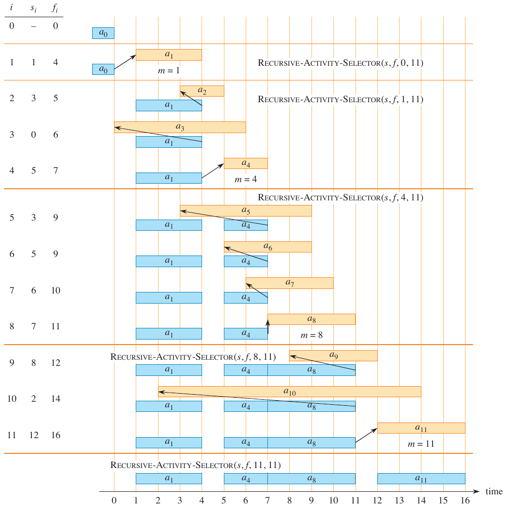
Figure 2: Recursive activity selector example (Cormen et al. 2022).
Analysis
At first glance, the algorithm appears to be \(O(n^2)\) because of the while loop coupled with the recursive call. Once an activity has been selected, the recursive call only considers the activities next \(n - k\) activities. The while loop picks up where the previous call left off, so the total number of iterations is \(n\). The algorithm is \(O(n)\).
Iterative Algorithm
The above solution can be adapted to an iterative one.
def greedy_activity_selector(s, f):
    n = len(s) - 1
    A = [1]
    k = 1
    for m in range(2, n + 1):
        if s[m] >= f[k]:
            A.append(m)
            k = m
    return A
In the for loop, the first line essentially asks if \(a_m \in S_k\). If so, then add it to the solution set and update \(k\) to \(m\).
Analysis
The analysis of the iterative approach is much clearer. The loop goes over all activities once, so the algorithm is \(O(n)\).
Properties of Greedy Solutions
You can probably imagine a problem for which a greedy solution would not provide the optimal solution. Path planning is one such problem. If we greedily chose the shortest path at each step, we may have missed a shorter path that is not the shortest at each step. The activity selection problem just so happens to be a perfect candidate for a greedy solution, but what makes it so?
First, let’s review the major steps that led us to the greedy solution for activity selection.
- Determine the optimal substructure.
- Develop a recursive solution.
- Show that making the greedy choice leaves only a single subproblem.
- Prove that making the greedy choice leads to an optimal solution.
- Develop a recursive algorithm.
- Convert it to an iterative algorithm.
The first couple of steps are common to dynamic programming problems. In this case, we could have jumped straight to the greedy approach. Filtering out these extra steps leaves us with:
- Cast the optimization problem as one in which we make a choice and are left with a single subproblem.
- Prove that the greedy choice is optimal.
- Demonstrate optimal substructure: if you make a greedy choice, then you are left with a subproblem such that combining an optimal solution with the greedy choice made previously, you end up with an optimal solution to the original problem.
As we will see, we need two properties to prove that a greedy solution is optimal: the greedy choice property and the optimal substructure property.
Greedy Choice Property
The greedy choice property states that the optimal solution can be found by making locally greedy choices. This approach is opposite of dynamic programming, where the choices at each step are made from the knowledge of optimal solutions to subproblems. That is, dynamic programming is a bottom-up approach.
A greedy solution also makes a choice at each step, but it is only based on local information. This is a top-down approach. They key of this property is to show that the greedy choice is optimal at each step. For the activity selection problem, the steps were
- Examine the optimal solution.
- If it has the greedy choice, then the greedy choice is optimal.
- If it does not have the greedy choice, then replace the suboptimal choice with the greedy choice.
Optimal Substructure Property
A problem has optimal substructure if the optimal solution contains optimal solutions to subproblems. We demonstrated this earlier for activity selection. We can start with the assumption that we arrived to a subproblem by making greedy choices. The next step is to show that the optimal solution to the subproblem combined with the greedy choice leads to an optimal solution to the original problem.
Greedy vs. Dynamic Programming
Since there is such overlap between greedy algorithms and dynamic programming in terms of their properties, it is important to understand the differences between the two. To illustrate these difference, we will look at two variations of the same problem.
\(0-1\) Knapsack Problem
Consider the \(0-1\) knapsack problem.
- You have \(n\) items.
- Item \(i\) is worth \(v_i\) and weighs \(w_i\).
- Find the most valuable subset of items with total weight less than or equal to \(W\).
- Items cannot be divided.
If the most valuable subset of items weighing at most \(W\) includes item \(j\), then the remaining weight must be the most valuable subset of items weighing at most \(W - w_j\) taken from \(n-1\) original items excluding item \(j\).
Fractional Knapsack Problem
This is similar to the \(0-1\) knapsack problem, but items can be divided. The objective is to maximize the value of the items in the knapsack.
The optimal substructure of this problem varies slightly: if the most valuable subset weighing at most \(W\) includes the weight \(w\) of item \(j\), then the remaining weight must be the most valuable subset weighing at most \(W- w\) that can be taken from the \(n-1\) original items plus \(w_j - w\) of item \(j\). There is some fraction of item \(j\) left after taking \(w\) of it.
Showing the Greedy Property
It is established that both problems have optimal substructure. However, only the fractional knapsack problem has the greedy property. Examine the following code:
def fractional_knapsack(v, w, W):
    n = len(v)
    load = 0
    i = 0
    while load < W and i <= n:
        if w[i] <= W - load:
            load += w[i]
            i += 1
        else:
            load += (W - load) * v[i] / w[i]
If we are able to sort each item by its value-to-weight ratio, then the greedy choice is to take as much as possible from the most valuable item first, the second most valuable item next, and so on. This considers \(n\) items in the worst case, and the items need to be sorted by value-to-weight ratio. The algorithm is \(O(n \log n)\).
This does not work for the \(0-1\) knapsack problem. Consider the problem visualized below.
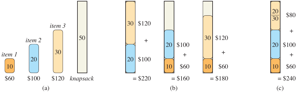
Figure 3: Greedy solution to the (0-1) knapsack problem (Cormen et al. 2022).
In this problem, we have a knapsack whose total capacity is \(W = 50\). A table of the weights, values, and value-to-weight ratios is given below.
| \(i\) | 1 | 2 | 3 |
|---|---|---|---|
| \(v_i\) | 60 | 100 | 120 |
| \(w_i\) | 10 | 20 | 30 |
| \(v_i/w_i\) | 6 | 5 | 4 |
The fractional algorithm would selection the first item since it has the greatest value-to-weight ratio. The \(0-1\) knapsack problem, however, would select the second and third items to maximize the value of the items in the knapsack.
Huffman Codes
Huffman coding is a lossless data compression algorithm that assigns variable-length codes to input characters, with lengths based on the frequencies of occurrence for those characters. Originally developed by David A. Huffman in 1952 during his Ph.D. at MIT, he published the algorithm under the title “A Method for the Construction of Minimum-Redundancy Codes”.
Huffman coding involves:
- Building a Huffman tree from the input characters and their frequencies.
- Traversing the tree to assign codes to each character.
Before getting into the specifics of the algorithm, let’s look at an example. Suppose we have a document consisting of 6 unique characters, each represented by a byte (8 bits). We could represent these 6 characters using 3 bits, since that is the minimum number of bits needed to represent 6 unique values. This is known as a fixed-length code. If we instead assigned a variable-length code to each character based on its frequency of occurrence, we would further reduce the footprint of the file size.
| A | B | C | D | E | F | |
|---|---|---|---|---|---|---|
| Frequency (in thousands) | 45 | 13 | 12 | 16 | 9 | 5 |
| Fixed-length code | 000 | 001 | 010 | 011 | 100 | 101 |
| Variable-length code | 0 | 101 | 100 | 111 | 1101 | 1100 |
- Does this seem like the best coding?
- Why isn’t a code of 1 used?
- What about 2 bit encoding?
The truth is that it depends on the document being compressed. The encoding is optimal considering the overall but length of the encoded file. Based on the above fixed-length code, the file size is 300,000 bits. The variable-length code reduces the file size to 224,000 bits.
How many bits are needed to encode \(n \geq 2\) characters?
\[ \lceil \lg n \rceil \]
Prefix-free Codes
A prefix-free code is a code in which no codeword is also a prefix of another codeword. This property simplifies decoding since the code can be read from left to right without ambiguity. The codeword “beef” has the encoding \(101110111011100 = 101 \cdot 1101 \cdot 1101 \cdot 1100\), where \(\cdot\) denotes concatenation.
This definition may start to clarify why a code of 1 is not used. If a code of 1 were used, then the code would be a prefix of all other codes. This would make decoding ambiguous.
How are the codes decoded?
One solution to this is to keep a table of all codewords and their corresponding characters. A more compact solution is to use a binary tree. Starting with the first bit in the encoded message, traverse the tree until a leaf node is reached. The character at the leaf node is the decoded character. The tree is known as a Huffman tree.
A full binary tree, where each nonleaf node has two subnodes, is optimal for decoding. If the tree has this property then an optimal prefix-free code has \(|C|\) leaves and exactly \(|C| - 1\) internal nodes. The tree for the variable-length code is shown below.
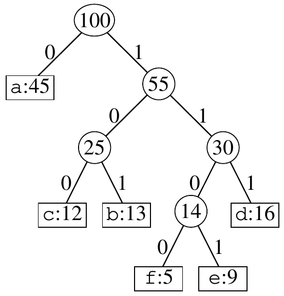
Figure 4: Huffman tree for the variable-length code (Cormen et al. 2022).
Given a character \(c\) with frequency \(c.freq\), let \(d_T( c)\) denote the depth of character \(c\) in tree \(T\). The cost of the code in bits is given by
\[ B(T) = \sum_{c \in C} c.freq \cdot d_T( c). \]
The depth of the character \(d_T( c)\) is used since it also denotes the length of the codeword.
Constructing a Huffman Code
class Node:
    def __init__(self, freq, char=None):
        self.freq = freq
        self.char = char
        self.left = None
        self.right = None

def huffman(C):
    n = len(C)
    Q = build_min_heap(C)
    for _ in range(n - 1):
        z = Node(0)
        z.left = x = extract_min(Q)
        z.right = y = extract_min(Q)
        z.freq = x.freq + y.freq
        insert(Q, z)
    return extract_min(Q)
The function above builds a Huffman tree from a set of characters \(C\). At each iteration, the two nodes with the smallest frequencies are extracted from the queue \(Q\) and are used to create a new node \(z\). This node represents the sum of the frequencies of the two nodes. The node is then inserted back into the queue so that it can be used in future iterations. The result is a Huffman tree.
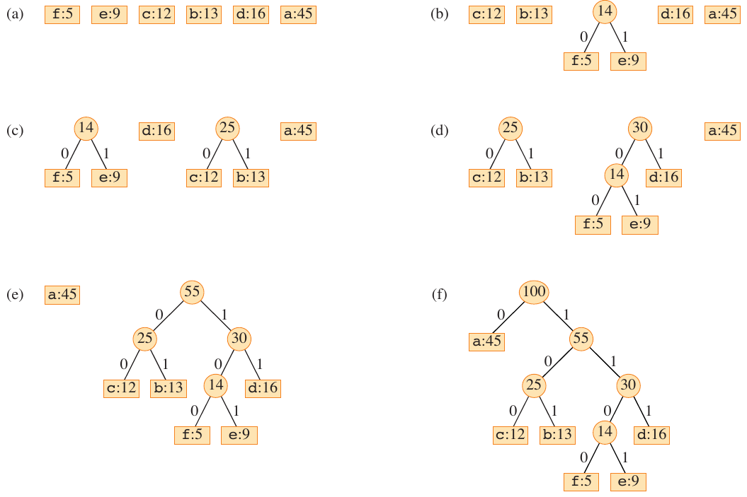
Figure 5: Huffman tree for the data in the table above (Cormen et al. 2022).
Analysis
If the priority queue is implemented as a binary min-heap, the call to build_min_heap initializes the priority queue in \(O(n)\) time. The for loop runs \(n-1\) times, calling extract_min twice and insert once. Each call to extract_min takes \(O(\lg n)\) time yielding a total of \(O(n \lg n)\) time.
Correctness of Huffman Codes
The correctness of an algorithm means that it produces the expected output based on the input and its properties. To show that the Huffman algorithm is correct, we can show that it exhibits the greedy choice and optimal substructure properties.
Lemma 15.2: Optimal prefix-free codes have the greedy-choice property
For alphabet \(C\), let \(x\) and \(y\) be the two characters with the lowest frequencies. Then there exists an optimal prefix-free code for \(C\) where the codewords for \(x\) and \(y\) have the same length and differ only in the last bit.
This establishes the greedy choice property because the algorithm selects the two characters with the lowest frequencies at each step.
Proof
In the given optimal tree \(T\), leaves \(a\) and \(b\) are two siblings with maximum depth. It’s also given that \(x\) and \(y\) are the two characters with the lowest frequencies, but they appear in arbitrary positions.
Assume that \(x \neq b\). Swapping \(a\) and \(x\) produces tree \(T’\) does not increase the cost. Swapping \(b\) and \(y\) produces tree \(T’’\) that also does not increase the cost. This is the key argument: if swapping the lowest frequency characters with the deepest characters does not increase the cost, then the greedy choice is optimal.
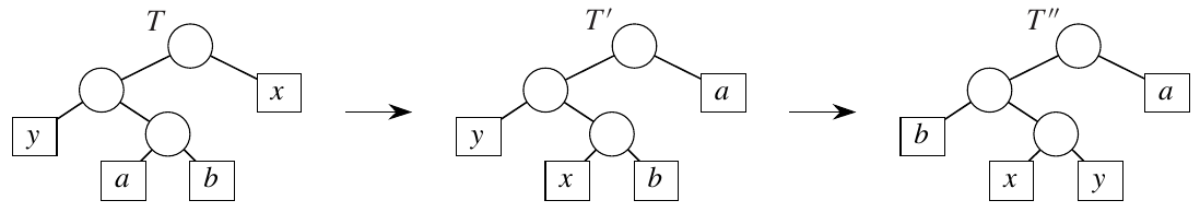
Figure 6: Creating (T’) and (T’’) from (T) (Cormen et al. 2022).
Next, we need to show that exchanging \(a\) and \(x\) does not increase the cost. The cost of the tree is given by
\[ B(T) = \sum_{c \in C} c.freq \cdot d_T( c). \]
\begin{align*} B(T) - B(T’) &= \sum_{c \in C} c.freq \cdot d_{T}( c) - \sum_{c \in C} c.freq \cdot d_{T’}( c) \\ &= x.freq \cdot d_T(x) + a.freq \cdot d_T(a) - x.freq \cdot d_{T’}(x) - a.freq \cdot d_{T’}(a) \\ &= x.freq \cdot d_T(x) + a.freq \cdot d_T(a) - x.freq \cdot d_{T}(a) - a.freq \cdot d_{T}(x) \\ &= (x.freq - a.freq)(d_T(x) - d_T(a)) \\ &\geq 0. \end{align*}
The last line is true because \(x.freq \leq a.freq\) and \(d_T(x) \geq d_T(a)\). A similar argument can be made for \(T’’\). \(B(T’’) \leq B(T’)\) since exchanging \(y\) and \(b\) does not increase the cost. This means that \(B(T’’) \leq B(T’) \leq B(T)\). \(T\) is an optimal tree, so \(B(T) \leq B(T’’) \implies B(T) = B(T’’) \implies T\) is optimal where \(x\) and \(y\) are siblings of maximum depth.
Lemma 15.3: Optimal-substructure property
Let \(x\) and \(y\) be two characters with minimum frequency in alphabet \(C\) and let \(C’ = (C - \{x, y\}) \cup z\) for a new character \(z\) with \(z.freq = x.freq + y.freq\). Additionally, let \(T’\) be a tree representing an optimal prefix-free code for \(C’\), and \(T\) be \(T’\) with the leaf for \(z\) replaced by an internal node with children \(x\) and \(y\). Then \(T\) represents an optimal prefix-free code for \(C\).
Simplified: If the algorithm computed the optimal solution to the simplified problem, where \(z\) replaced \(x\) and \(y\), it can extend this to an optimal solution to the original problem by putting \(x\) and \(y\) back.
Proof
The first part of the proof establishes the costs of the relevant trees.
\(c \in C - \{x, y\} \implies d_T( c) = d_{T’}( c) \implies c.freq \cdot d_T( c) = c.freq \cdot d_{T’}( c)\)
The depth of \(x\) and \(y\) are equal to the depth of \(z\) in \(T’\) + 1:
\begin{align*} d_T(x) = d_T(y) = d_{T’}(z) + 1 &\implies x.freq \cdot d_T(x) + y.freq \cdot d_T(y)\\ &= (x.freq + y.freq)(d_{T’}(z) + 1)\\ &= z.freq \cdot d_{T’}(z) + (x.freq + y.freq). \end{align*}
This means that \(B(T) = B(T’) + x.freq + y.freq\), which is equivalent to \(B(T’) = B(T) - x.freq - y.freq\).
The second part of this proof supposes that \(T\) is not an optimal prefix code for \(C\) and ends in a contradiction, thus proving the original lemma. If \(T\) is not optimal for \(C\), then \(B(T’’) < B(T)\) for some optimal tree \(T’’\).
Here, \(T’’\) is introduced as the supposed optimal tree for \(C\) if it turns out that \(T\) is not.
If \(T’’\) is optimal, then lemma 15.2 (greedy property) from above implies that it has \(x\) and \(y\) as siblings. After all, \(\{x, y\} \in C\) and \(T’’\) is an optimal tree for \(C\). Create a tree \(T’’’\) by replacing the parent of \(x\) and \(y\) with a leaf (implying we remove \(x\) and \(y\)) \(z\) with \(z.freq = x.freq + y.freq\). Then,
\begin{align*} B(T’’’) &= B(T’’) - x.freq - y.freq\\ &< B(T) - x.freq - y.freq\\ &= B(T’). \end{align*}
\(B(T’’’) < B(T’)\) is a contradiction because it was previously established that \(T’\) is an optimal tree for \(C’\). Therefore a suboptimal \(T\) is impossible if \(T’\) is optimal.