Hidden Markov Models
Introduction
This article is essentially a grok of a tutorial on HMMs by (RABINER 1989). It will be useful for the reader to reference the original paper.
Up to this point, we have only explored “atomic” data points. That is, all of the information about a particular sample is encapsulated into one vector. Sequential data is easily represented by graphical models. This article introduces Hidden Markov Models, a powerful probabilistic graphical model used in many applications from gesture recognition to natural language processing.
There are many tasks for which we do not know the underlying process. However, we can observe samples that are produced from such processes. Music, gesture recognition, speech, text, etc. All of these have some underlying process which forms their outputs together into a hopefully coherent sequence. If we wish to make predictions about future samples given these sequences, we will need to make some guess about the underlying processes defining their output.
The Markov Assumption
Markov models make a convenient assumption about sequential data. That is, all relevant information required for predicting future samples is captured in the current time step \(t\). Given a joint distribution over an input of \(T\) frames, \(p(\mathbf{x}_{1:T})\), the Markov assumption allows us to represent it as
\[ p(\mathbf{x}_{1:T}) = p(\mathbf{x}_1)\prod_{t=2}^T p(\mathbf{x}_t|\mathbf{x}_{t-1}) \]
Definition
A more complicated case is when we are attempting to model some unknown process that is responsible for the observations. In this case, an ordinary Markov chain is not sufficient. A hidden Markov model (HMM) is defined by a set \(z_t \in \{1, \dots, K\}\) of discrete hidden states and an observation model \(p(\mathbf{x}_i|z_t)\). The joint probability distribution of this model is given by
\[ p(\mathbf{z}, \mathbf{x}) = p(\mathbf{z})p(\mathbf{x}|\mathbf{z}) = \Big(p(z_1)\prod_{t=2}^Tp(z_t|z_{t-1})\Big)\Big(\prod_{t=1}^Tp(\mathbf{x}_t|z_t)\Big). \]

Figure 1: The observations y are generated by the latent states x. Source: Wikipedia
Although the states themselves are discrete, the observations may be continuous: \(p(\mathbf{x}|z_t, \mathbf{\theta})\). If they are discrete, they can be modeled by an observation matrix \(B\). Continuous observations are typically modeled using a conditional Gaussian:
\[ p(\mathbf{x}_t|z_t=k, \theta) = \mathcal{N}(\mathbf{x}_t|\mathbf{\mu}_k,\mathbf{\Sigma}_k). \]
Following Rabiner, an HMM can be characterized by
- The number of states in the model \(N\).
- The number of distinct observation symbols per state \(M\).
- The state probability distribution \(A = \{a_{ij}\}\), \(a_{ij} = p(z_t=j | z_{t-1} = i)\).
- The observation symbol probability distribution \(B = \{b_j(k)\} = p(\mathbf{x}_t = k|z_t = j)\).
- An initial state distribution \(\mathbf{\pi}_i = p(z_t = i)\).
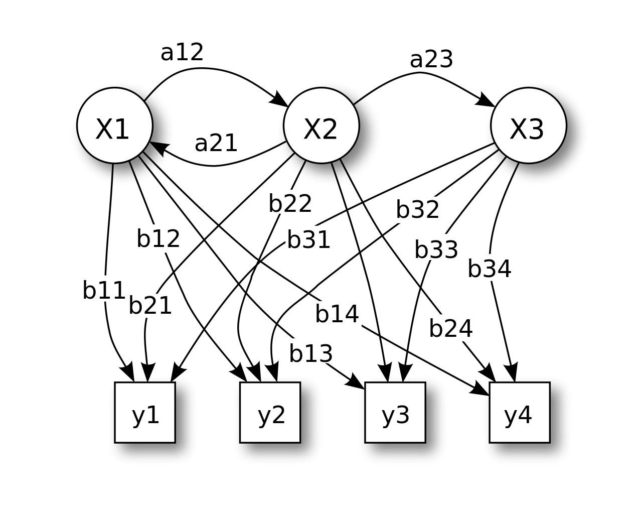
Figure 2: HMM with observation probabilities and state transition probabilities. Source: Wikipedia
The observation probability distribution is commonly modeled as a Gaussian, Mixture of Gaussians, or Multinomial distribution. Thus, the parameter estimates for those distributions follow the likelihood estimates for each respective distribution.
In his famous tutorial on HMMs, Rabiner addressed the three fundamental problems of HMMs:
- Given an observation sequence and model parameters, how do we compute the probability of the observation sequence given the parameters (likelihood)?
- Given an observation sequence and model parameters, how do we choose a state sequence which is optimal (decoding)?
- How do we adjust the model parameters (learning)?
HMMs are able to solve several different inference problems.
- Filtering computes \(p(z_t | \mathbf{x}_{1:t})\). That is, we are computing this probability as new samples come in up to time \(t\).
- Smoothing is accomplished when we have all the data in the sequence. This is expressed as \(p(z_t|\mathbf{x}_{1:T})\).
- Fixed lag smoothing allows for a trade off between accuracy and delay. It is useful in cases where we might not have the full sequence, but we wish to compute \(p(z_{t-l}|\mathbf{x}_{1:t})\) for some \(l > 0\).
- Predictions are represented as \(p(z_{t+h}|\mathbf{x}_{1:t})\), where \(h > 0\).
- MAP estimation yields the most probably state sequence \(\text{arg}\max_{\mathbf{z}_{1:T}}p(\mathbf{z}_{1:T}|\mathbf{x}_{1:T})\).
- We can sample the posterior \(p(\mathbf{z}_{1:T}|\mathbf{x}_{1:T})\).
- We can also compute \(p(\mathbf{x}_{1:T})\) by summing up over all hidden paths. This is useful for classification tasks.
Evaluation
We start by solving the first problem posited by (RABINER 1989).
- Given an observation sequence and model parameters, how do we compute the probability of the observation sequence given the parameters?
That is, given some model parameters \(\lambda = (A, B, \pi)\), compute \(p(z_t|\mathbf{x}_{1:t})\).
Forwards Pass
The forwards algorithm solves two problems of interest. First, we want to know how well our current parameters explain the observation sequence. That is, \(p(\mathbf{x}_{1:T}|\lambda)\).
Second, we want to compute \(p(z_t | \mathbf{x}_{1:t})\). To compute these in an efficient way, a recursive strategy is adopted. Let the forward variable \(\alpha_t(i)\) be defined as
\[ \alpha_t(i) = p(\mathbf{x}_{1:t}, z_t = i | \lambda). \]
The forwards algorithm is defined as 3 steps.
-
Initialization:
\[ \alpha_1(i) = \pi_i b_i(\mathbf{x}_1),\quad 1 \leq i \leq N. \]
-
Recursion:
\[ \alpha_{t+1}(j) = \Big(\sum_{i=1}^N \alpha_t(i)a_{ij}\Big)b_j(\mathbf{x}_{t+1}),\quad 1 \leq t \leq T - 1,\quad 1 \leq j \leq N \]
-
Termination:
\[ p(\mathbf{x}_{1:T}) = \sum_{i=1}^N \alpha_T(i). \]
The recursive step is visualized as a lattice structure as seen below.
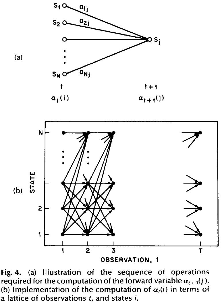
Figure 3: From Rabiner 1989.
With this step, we have a solution for the first problem. We can now calculate more efficiently the probability of our observations given the current model parameters. This along with the following backwards pass will be essential for updating our model parameters.
The forwards algorithm is also used to solve the filtering problem. To see how, consider \(p(z_t | \mathbf{x}_{1:t-1})\) right before time \(t\).
\begin{equation*} p(z_t=j|\mathbf{x}_{1:t-1}) = \sum_i p(z_t=j|z_{t-1}=i)p(z_{t-1}=i|\mathbf{x}_{1:t-1}) \end{equation*}
When we update for time \(t\), we have that
\begin{align*} p(z_t=j|\mathbf{x}_{1:t}) &= p(z_t=j|\mathbf{x}_t, \mathbf{x}_{1:t})\\ &=\frac{p(\mathbf{x}_t|z_t=j, \mathbf{x}_{1:t-1})p(z_t=j|\mathbf{x}_{1:t-1})}{p(\mathbf{x}_t|\mathbf{x}_{t-1})} \end{align*}
However, \(\mathbf{x}_{1:t-1}\) is conditionally independent given \(z_t\), so it becomes
\begin{equation*} p(z_t=j|\mathbf{x}_{1:t})=\frac{p(\mathbf{x}_t|z_t=j)p(z_t=j|\mathbf{x}_{1:t-1})}{p(\mathbf{x}_t|\mathbf{x}_{t-1})}. \end{equation*}
Writing out \(p(z_t=j|\mathbf{x}_{1:t-1})\) fully yields
\begin{equation*} p(z_t=j|\mathbf{x}_{1:t}) \propto p(\mathbf{x}_t|z_t=j)\sum_i p(z_t=j|z_{t-1}=i)p(z_{t-1}=i|\mathbf{x}_{1:t-1}). \end{equation*}
This is the recursion step from above!
This can also be represented in terms of the \(\alpha\) variables from above. To compute \(p(z_t=i|\mathbf{x}_{1:t})\), we can use the definition of a conditional probability distribution:
\begin{align*} p(z_t=i|\mathbf{x}_{1:t}) &= \frac{p(z_t=i, \mathbf{x}_{1:t})}{p(\mathbf{x}_{1:t})}\\ &= \frac{\alpha_t(i)}{\sum_{j=1}^N \alpha_t(j)} \end{align*}
Compared to the complexity of the explicit representation, the forwards pass needs only \(N^2T\) calculations. As pointed out in (RABINER 1989), with 5 hidden states and an observation sequence of length 100, the forwards pass only needs around 3000 computations. A direct calculation would require \(10^{72}\).
Backwards Pass
When updating the parameters of our model, we will need to consider the entire observation sequence. The forward pass did not require the entire sequence. Instead, we can compute the probability of the observation up to some time \(t\). The backwards pass begins by defining the variable
\[ \beta_t(i) = p(\mathbf{x}_{t+1:T} | z_t = i). \]
We can utilize a recursive process similar to the forwards algorithm with the following steps:
-
Initialization:
\[ \beta_T(i) = 1,\quad 1 \leq i \leq N \]
-
Recursion:
\[ \beta_t(i) = \sum_{j=1}^N a_{ij}b_j(\mathbf{x}_{t+1})\beta_{t+1}(j),\quad t = T-1,\dots,1,\quad 1 \leq i \leq N. \]
-
Termination:
\[ p(\mathbf{x}_{1:T}) = \sum_{j=1}^N \pi_j b_j(x_1) \beta_1(j) \]
The complexity of the backwards algorithm is similar to that of the forwards: \(N^2T\).
With both the forward and backwards passes defined, we can compute the smoothing problem:
\[ p(z_t=i|\mathbf{x}_{1:T}) = \frac{\alpha_t(i)\beta_t(i)}{\sum_{j=1}^N \alpha_t(j)\beta_t(j)} \]
The Viterbi Algorithm
With problem 1 out of the way, we turn our attention to problem 2.
- Given an observation sequence and model parameters, how do we choose a state sequence which is optimal?
\[ \mathbf{z}^* = \text{arg}\max_{\mathbf{z}_{1:T}}p(\mathbf{z}_{1:T}|\mathbf{x}_{1:T}) \]
With respect to the lattice diagram, this is equivalent to computing the shortest path. This is accomplished via the Viterbi algorithm, sometimes referred to as the max-sum algorithm. As with the forwards-backwards algorithm, the Viterbi algorithm takes on a recursive approach. It starts by defining an intermediate variable
\[ \gamma_t(i) = p(z_t=i|\mathbf{x}_{1:T}). \]
Using the variables defined in the forwards-backwards algorithm, this can be expressed as
\[ \gamma_t(i) = \frac{\alpha_t(i) \beta_t(i)}{\sum_{i=1}^N \alpha_t(i) \beta_t(i)}. \]
This \(\gamma_t(i)\), we can compute the most likely state at time \(t\):
\[ z_t^* = \text{arg}\max_{1\leq i \leq N} \gamma_t(i), \quad 1 \leq t \leq T. \]
One problem with this approach alone is that the most likely state at a particular time \(t\) may not lead us to the most probable sequence of states. As stated above, we need to maximize \(p(\mathbf{z}_{1:T}|\mathbf{x}_{1:T})\). In order to tackle this efficiently, Viterbi employs a dynamic programming approach.
-
Initialization
Start with the best initial state out of all states given the observation at \(t=1\). Additionally, we want to record the index of each state through time so that the best path can be retraced.
\begin{align*} \delta_1(i) &= \pi_i b_i(\mathbf{x}_1),\quad 1 \leq i \leq N\\ \psi_1(i) &= 0 \end{align*}
-
Recursion:
The quantity \(\delta_t(i)\) represents the joint probability of state sequences and observations up to time \(t\) ending with state \(z_t=i\). Thus, the recursive step is to maximize the probability of the intermediate output for \(t-1\):
\[ \delta_t(j) = \max_{1 \leq i \leq N} (\delta_{t-1}(i) a_{ij})b_j(\mathbf{x}_t), \quad 2 \leq t \leq T,\quad 1 \leq j \leq N. \]
The corresponding index for this step is recorded in the path matrix:
\[ \psi_t(j) = \text{arg}\max_{1 \leq i \leq N} \delta_{t-1}(i)a_{ij},\quad 2 \leq t \leq T,\quad 1 \leq j \leq N. \]
-
Termination
The last step of the Viterbi algorithm completes the calcuation of the joint probability of state sequences and observations.
\[ p^* = \max_{1 \leq i \leq N} \delta_T(i) \]
\[ \mathbf{z}_T^* = \text{arg}\max_{1 \leq i \leq N} \delta_T(i) \]
-
Path Backtrace
With the state sequence matrix recorded along the way, we can retrace it to get the most probable sequence:
\[ z_t^* = \psi_{t+1}(z_{t+1}^*),\quad t = T-1, \cdots, 1. \]
Estimating Parameters
If the hidden states were fully observable, then updating our model parameters would be as straightforward as computing the maximum likelihood estimates for the model parameters \(\lambda = (A, B, \pi)\). For \(A\) and \(\pi\), we first tally up the following counts:
\[ \hat{a}_{ij} = \frac{N_{ij}}{\sum_j N_{ij}}, \]
the number of times we expect to transition from \(i\) to \(j\) divided by the number of times we transition from \(i\) to any other state.
For \(\pi\), we have
\[ \hat{\pi_i} = \frac{N_i}{\sum_i N_i}, \]
The number of times we expect to start in state \(i\) divided by the number of times we start in any other state.
Estimating the parameters for \(B\) depends on which distribution we are using for our observation probabilities. For a multinomial distribution, we would compute the number of times we are in state \(j\) and observe a symbol \(k\) divided by the number of times we are in state \(j\):
\[ \hat{B}_{jk} = \frac{N_{jk}}{N_k}, \]
where
\[ N_{jk} = \sum_{i=1}^N \sum_{t=1}^T \mathbb{1} (z_{i, t}=j, x_{i, t}=k). \]
If the observation probability follows a Gaussian distribution, the MLEs for \(\mu\) and \(\mathbf{\Sigma}\) are
\[ \hat{\mathbf{\mu}}_k = \frac{\bar{\mathbf{x}}_k}{N_k},\quad \hat{\mathbf{\Sigma}}_k = \frac{(\bar{\mathbf{x}}\bar{\mathbf{x}})_k^T - N_k \hat{\mathbf{\mu}}_k\hat{\mathbf{\mu}}_k^T}{N_k}, \]
where
\[ \bar{\mathbf{x}}_k = \sum_{i=1}^N \sum_{t=1}^T \mathbb{1}(z_{i, t}=k)\mathbf{x}_{i, t} \]
and
\[ (\bar{\mathbf{x}}\bar{\mathbf{x}})_k^T) = \sum_{i=1}^N \sum_{t=1}^T \mathbb{1} (z_{i, t}=k)\mathbf{x}_{i,k}\mathbf{x}_{i,k}^T. \]
Expectation Maximization
Of course, HMMs have hidden states which are not fully observable. Thus, we need to come up with another strategy for updating our parameters based on the observable data. The intuition behind this approach is as follows. We first start out by using our current parameters to estimate the missing data, making it complete. Initially, we may randomize our estimates if we have no good heuristic or guess as to what they should be.
With the completed data, we can update our current parameters. In other words, the expected values of the sufficient statistics can be derived now that the data has been filled in. A new set of parameters is found such that it maximizes the likelihood function with respect to the estimated data.
E Step
Following (RABINER 1989), we start with the joint probability of being in state \(i\) at time \(t\) and state \(j\) at time \(t+1\):
\[ \xi_t(i, j) = p(z_t = i, z_{t+1} = j|\mathbf{x}_{1:T}). \]
This can be computed using the forwards-backwards algorithm:
\[ \xi_t(i, j) = \frac{\alpha_t(i)a_{ij}b_j(\mathbf{x}_{t+1})\beta_{t+1}(j)}{\sum_{i=1}^N \sum_{j=1}^N \alpha_t(i)a_{ij}b_j(\mathbf{x}_{t+1})\beta_{t+1}(j)}. \]
This can be related back to \(\gamma_t(i)\) by summing over over \(j\):
\[ \gamma_t(i) = \sum_{j=1}^N \xi_t(i, j). \]
Here, \(\gamma_t(i)\) is the expected number of times we transition from \(z = i\). Summing over all \(t\) yields the expected transitions from \(z_i\) over all time steps:
\[ \sum_{t=1}^{T-1} \gamma_t(i). \]
Since \(\xi_t(i, j)\) is the expected transition from \(i\) to \(j\) at time \(t\), we can compute the total number of transitions from \(i\) to \(j\) via
\[ \sum_{t=1}^{T-1} \xi_t(i, j). \]
M Step
The previous E Step computed the expected values given the current parameter estimates. Now that the data is complete, we can update our parameter estimates. Starting with the transition probabilities, we must add the expected number of transitions from \(i\) to \(j\) and divide by the expected number of times we transition from \(i\). Using the parameters from the E Step, this can be written
\[ \hat{a}_{ij} = \frac{\sum_{t=1}^{T-1}\xi_t(i, j)}{\sum_{t=1}^{T-1}\gamma_t(i)}. \]
The initial state probability at \(t=1\) is the number of times we expect to be in state \(z=i\) at \(t=1\):
\[ \gamma_1(i). \]
Finally, the observation probability parameters are updated by considering the number of times we are in state \(z=j\) and observing \(x=k\) divided by the number of times we are in state \(z=j\). Note that this is for a multinomial probabiliy distribution:
\[ \hat{b}_j(k) = \frac{\sum_{t=1, x_t = k}^T \gamma_t(j)}{\sum_{t=1}^T \gamma_t(j)}. \]
These formulas are derived from maximizing Baum’s auxiliary function
\[ Q(\lambda, \hat{\lambda}) = \sum_{Q} p(\mathbf{z}|\mathbf{x}, \lambda) \log p(\mathbf{x}, \mathbf{z}|\hat{\lambda}) \]
over \(\hat{\lambda}\). It has further been shown that maximizing this function leads to increased likelihood:
\[ \max_{\hat{\lambda}} Q(\lambda, \hat{\lambda}) \implies p(\mathbf{x}|\hat{\lambda}) \geq p(\mathbf{x}|\lambda). \]
If we have a Gaussian observation model, the values for \(\hat{b}_j(k)\) are computed to accommodate the parameters of the distribution. These parameter estimates assume a Gaussian mixture model. Starting with \(\hat{\mu}_{jk}\), it can be estimated by dividing the expected value of observations belonging to Gaussian density \(k\) by the expected number of times we are in state \(j\) using the \(k^{\text{th}}\) mixture component:
\[ \hat{\mathbf{\mu}}_{jk} = \frac{\sum_{t=1}^T \gamma_t(j, k)\mathbf{x}_t}{\sum_{t=1}^T \gamma_t(j, k)}. \]
Here, \(\gamma_t(j, k)\) is the probability of being in state \(j\) at time \(t\) with the \(k^{\text{th}}\) mixture component accounting for \(\mathbf{x}_t\):
\[ \gamma_t(j, k) = \frac{\alpha_t(j)\beta_t(j)}{\sum_{j=1}^N \alpha_t(j) \beta_t(j)} \frac{c_{jk}\mathcal{N}(\mathbf{x}_t, \mu_{jk}, \mathbf{\Sigma}_{jk})}{\sum_{m=1}^M c_{jm}\mathcal{N}(\mathbf{x}_t, \mu_{jm}, \mathbf{\Sigma}_{jm})}. \]
This method is proven to improve the parameters.
- Each iteration is guaranteed to improve the log-likelihood function.
- The process is guaranteed to converge.
- The convergence point is a fixed point of the likelihood function.
These guarantees are similar to gradient ascent.