Histogram of Oriented Gradients
Introduction
Key Questions
- Why are these necessary?
- What limitations do they address that corner interest points cannot?
Although the original HOG Paper came out after SIFT, it is much simpler to describe the process (Dalal and Triggs 2005). Histograms of Oriented Gradients are feature vectors that are generated by evaluating gradients within a local neighborhood of interest points.
Orientation Histograms
This approach depends on building orientation histograms. For each pixel in the original image, construct a histogram of gradient orientations of all pixels within a square window. The gradient orientations of each pixel are easily calculated following the approach used for Edge Detection. This transformation can be flattened into a single vector that is used to compare images via L2 distance or some other metric.
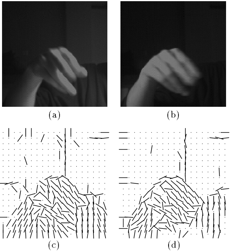
Figure 1: Orientation histograms of hand images.
The pseudocode to generate orientation histograms is shown below.
let w be the window_size
let h be half the window_size
let norms be the gradient norms of the input image for each pixel
let angles be the computed orientations of the gradient vectors for each pixel
for each pixel (i, j):
    create a histogram of orientations with b bins
    weight the orientations of the bins based on the gradient norm
The histograms of each local feature are translation invariant. A histogram of gradient orientations for a feature in one image should be the same as one generated to a similar feature in another image.
This approach is not scale invariant.
Histogram of Oriented Gradients
Dalal and Triggs propose a feature extraction method based on orientation histograms (Dalal and Triggs 2005). In their work published at CVPR, they evaluate their features by training a SVM for pedestrian detection on a standard (at that time) benchmark. They evaluate on a person detector using the metric False Positives Per Window (FPPW). This can be calculated as num_fp / num_windows. This represents a tradeoff between the number of false positives and the number false negatives. Intuitively, lowering the threshold for detection will generate more false positives, but will also reduce the number of false negatives.
Computing HoG
- Normalize for color and gamma values.
- Compute the gradient image.
- Extract a window of some size.
- Divide window into sub-grid
- Compute orientation histogram of each cell.
- Concatentate the four histograms.
- Normalize the feature vector.
During the binning step, each pixel provides a weighted vote for the histogram based on the orientation of the gradient element it centered on. This vote is weighted based on a function of the gradient magnitude.
In the paper, they experiment with a wide range of different parameters. They show that optimal performance coincides with choosing 4 cells per window with 9 orientation bins.
Normalization Schemes
There were several normalizion schemes addressed in the paper.
The normalization scheme picked based on lowest FPPW is L2-Hys:
- Normalize the concatenated vector.
- Clip values to 0.2
- Normalize again.
They also evaulated the features with L2, L1, and L1-sqrt.
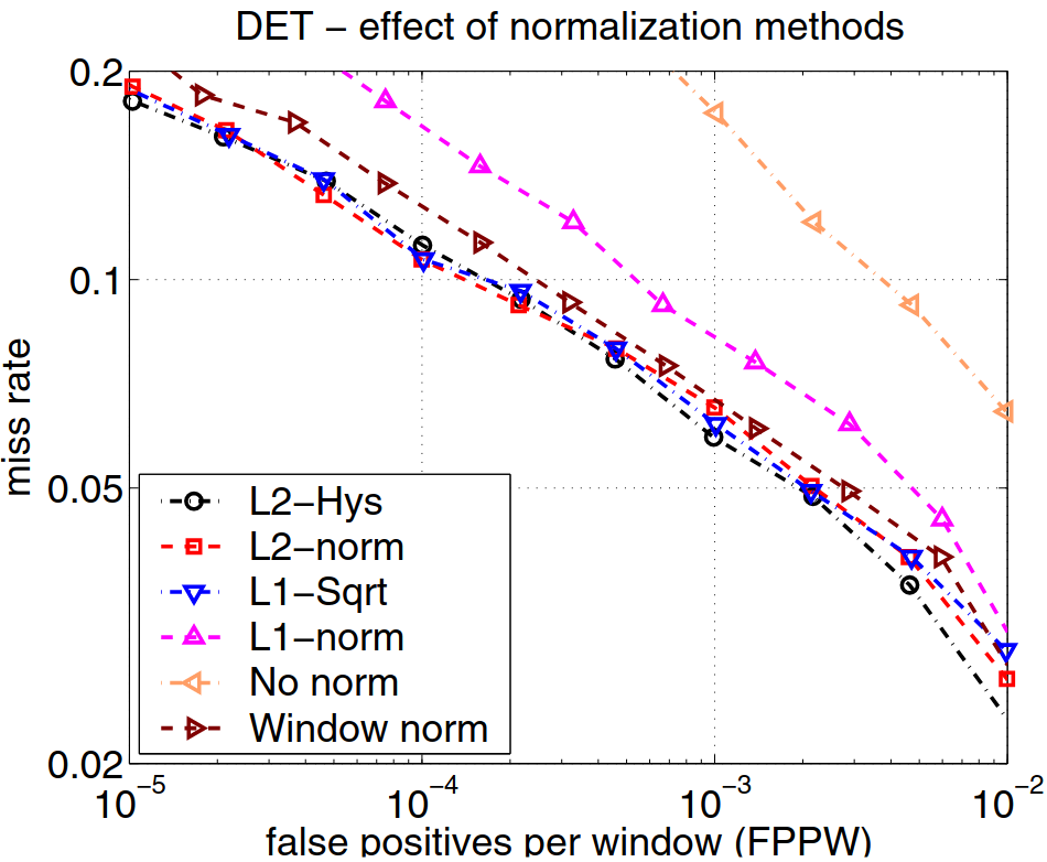
Figure 2: Evaluation of normalization approaches (Dalal and Triggs, 2005).