Hough Transform
Introduction
Fitting a model to a set of data by consensus, as in RANdom SAmple Consensus, produces a parameter estimate that is robust to outliers. A similar technique for detecting shapes in images is the Hough Transform. Originally it was designed for detecting simple lines, but it can be extended to detect arbitrary shapes.
The transform is computed given an edge image. Each edge pixel in the image casts a vote for a line given a set of parameters. This vote is added to an accumulator array which tallies the votes over all pixels for all parameter choices.
Algorithm
An accumulator array holds the votes for each edge point. The indices to this array represent the line parameters \((\rho, \theta)\), where
\[ \rho = x \cos \theta + y \sin \theta. \]
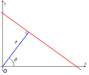
Figure 1: Parameterization of a line in a Hough transform. Source: Wikipedia
In this parameterization, \((\rho, \theta)\) represents a vector that is normal to the line. For each edge pixel in the original image, a range of \(\theta\) values are tested. The resolution of \(\theta\) values used is set as a hyperparameter to the algorithm. A vote is cast for every single line within the resolution of \(\theta\) by incrementing the accumulator array at entry \((\rho, \theta)\).
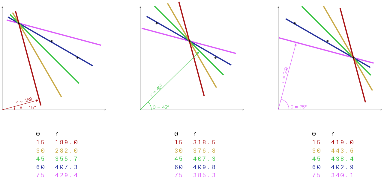
Figure 2: Visualization of voting procedure. Source: Wikipedia
After all edge pixels are evaluated, the accumulator array must be post processed to select the lines with the most agreement. Since the accumulator array is 2D, it can be visualized as seen below.
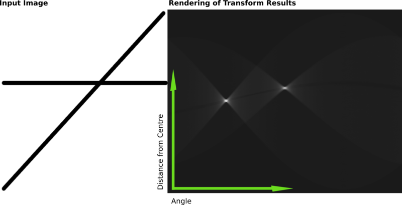
Figure 3: Visualization of accumulator array. Source: Wikipedia
Rectangle Detection based on a Windowed Hough Transform
As mentioned in the introduction, Hough transforms can be extended to detect arbitrary shapes. In their 2004 publication, Jung and Schramm approach the problem of detecting rectangles in an image via Hough transforms. By analyzing the spatial relationship of peaks in a standard Hough transform, rectangles can reliably be detected.
Detecting Rectangles via Hough peaks
If we consider pixel located at the center of a rectangle, a few key symmetries can be observed.
- The detected peaks from the Hough window will be in pairs, equidistant from the center.
- Two pairs will be separated by \(90^{\circ}\) with respect to the \(\theta\) axis.
- The distance between the peaks of a pair are the sides of the rectangle.
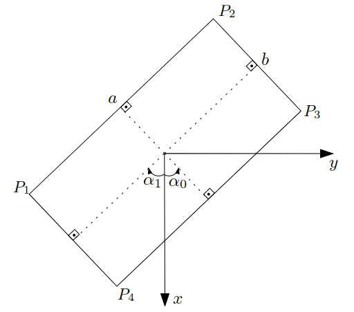
Figure 4: Rectangle centered at the origin.
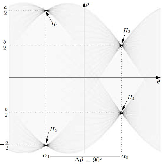
Figure 5: The resulting Hough transform of the previous figure.
The Algorithm
Each pixel in the image is evaluated using a sliding window approach. Consider a pixel centered on \((x_c, y_c)\). The size of the window determines the maximum size of the rectangle that can be detected in a given window. The authors use a circular threshold with a minimum and maximum diameter \(D_{min}\) and \(D_{max}\). That is, the search region is a circle such that the smallest detectable rectangle has a side length of no less than \(D_{min}\) and a diagonal length of no more than \(D_{max}\). The figure below visualizes this region.
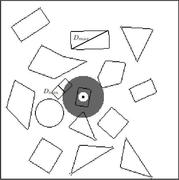
Figure 6: Search region based on a circle. Source: Jung and Schramm 2004.
With the search region defined, a hough transform for that region is computed. The paper mentions an optimization step when selecting the discretization steps \(d_{\theta}\) and \(d_{\rho}\). If the input image is large, the resulting Hough transform will also be large. They recommend picking \(d_{\theta} = \frac{3 \pi}{4 D_{max}}\) and \(d_{\rho} = \frac{3}{4}\).
The Hough image is further processed in order to extra local extrema. These peaks should correspond to the lines of the rectangle. First, an enhanced image is created following
\[ C_{\text{enh}}(\rho, \theta) = h w \frac{C(\rho, \theta)^2}{\int_{-h/2}^{h/2}\int_{-w/2}^{h/2} C(\rho + y, \theta + x)dx dy}. \]
How is such an integral computed? The integral is the “area under the curve” of a given signal. In this case, the accumulator image is a 2D signal for which a discrete approximation of the integral can be computed. This can be implemented via convolution. The local maxima of this enhanced image are those such that \(C(\rho, \theta) \geq T_C\), where \(T_C = 0.5D_{min}\).
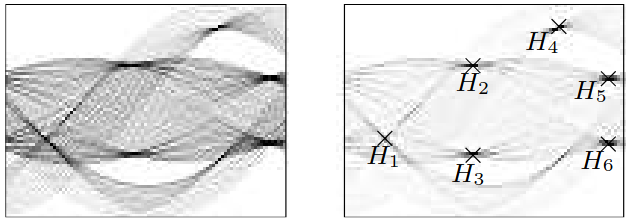
Figure 7: Original Hough image (left) and enhanced (right) (Jung and Schramm 2004).
With the detected peaks from the enhanced image, four peaks are selected with satisfy the symmetries of rectangles as listed above. This is shown as equation 3 in the paper:
\begin{align*} &\Delta \theta = |\theta_i - \theta_j| < T_{\theta},\\ &\Delta \rho = |\rho_i + \rho_j| < T_{\rho},\\ &|C(\rho_{i}, \theta_i) - C(\rho_j, \theta_j)| < T_{L}\frac{C(\rho_i, \theta_i) + C(\rho_j, \theta_j)}{2}. \end{align*}
\(T_{\theta}\) is used to threshold peaks corresponding to parallel lines (\(\theta_i \approx \theta_j\)). \(T_{\rho}\) is a threshold for symmetry (equal distance between lines and center). \(T_L\) ensures that line segments have approximately the same length.
For peaks that satisfy the equations above, an extended peak \(P_k = (\pm \xi, \alpha_k)\) is formed, where
\[ \alpha_k = \frac{1}{2}(\theta_i + \theta_j) \text{ and } \xi_k = \frac{1}{2}|\rho_i - \rho_j|. \]
Finally, a rectangle is detected if the pairs of lines are orthogonal. That is, if
\[ \Delta \alpha = ||\alpha_k - \alpha_l| - 90^{\circ}| < T_{\alpha}. \]
The rectangle parameters are encoded by \(\alpha_k\) being its orientation and \(2\xi_k\) and \(2\xi_l\) being its sides.
The final step in the paper is to remove duplicates since, depending on the threshold choices, multiple candidates for a rectangle may be detected. The intuition behind this step is to create an error measure that summarizes how well the symmetries defined by the conditions required for a rectangle are respected.
\[ E(P_k, P_l) = \sqrt{a(\Delta \theta_k^2 + \Delta \theta_l^2 + \Delta \alpha^2) + b(\Delta \rho_k^2 + \Delta \rho_l^2)} \]
In this error measure, \(a\) and \(b\) are used to weight the angular and distance errors differently since a change in 1 pixel would be more significant than a change of 1 degree.
If the difference in orientation for each line detected in the sides is greater, the orientation error increases. Likewise, the more that the pairs of lines stray from orthogonality, the greater the error becomes. For the distance measure, the more offset the lines are with respect to the center, the greater the error becomes. Thus, the rectangle that meets these criteria best will have the lowest error.