Image Features
Introduction
Why do we care about image features? One of the main goals of computer vision is understanding of some environment through visual perception. In order to summarize a visual object, we need some description of it. These descriptions can come in many forms, so we need to articulate some goals as to what we are ultimately looking for when describing an image.
What makes an interesting feature in an image?
- Something distinct
- Invariance properties (translation, rotation, scaling)
- Easy to compute
Image features are the building blocks of many higher level applications such as
- Stereo correspondence
- Image stitching
- Object recognition and detection
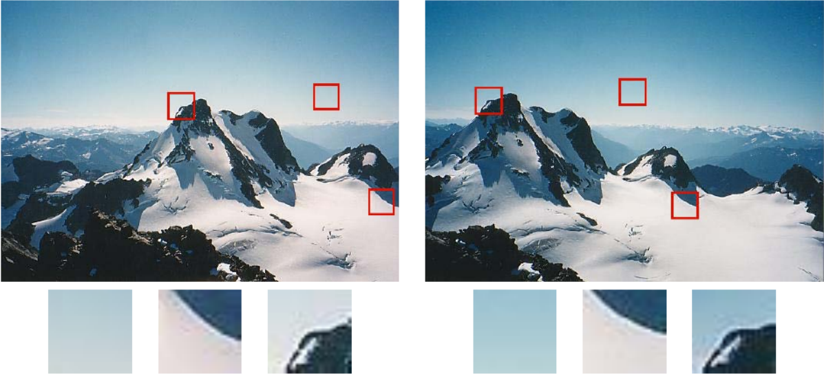
Figure 1: Patches taken from two images from different perspectives. Some patches are more descriptive than others. Source: Szeliski
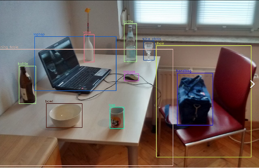
Figure 2: Objects detected using YOLOv3. Source: Wikipedia.
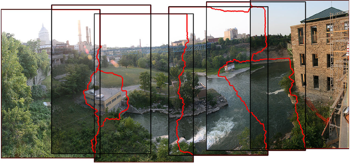
Figure 3: Image stitching result. The red lines show the seams at which the images are joined. Source: Wikipedia.
We have talked about Edge Detection, which produces an image of edge pixels given some raw input. Edges are certainly useful features, but are they distinct enough to produce consistent image features?
Consider an image patch detected from three different primitives:
- Points
- Edges
- Corners
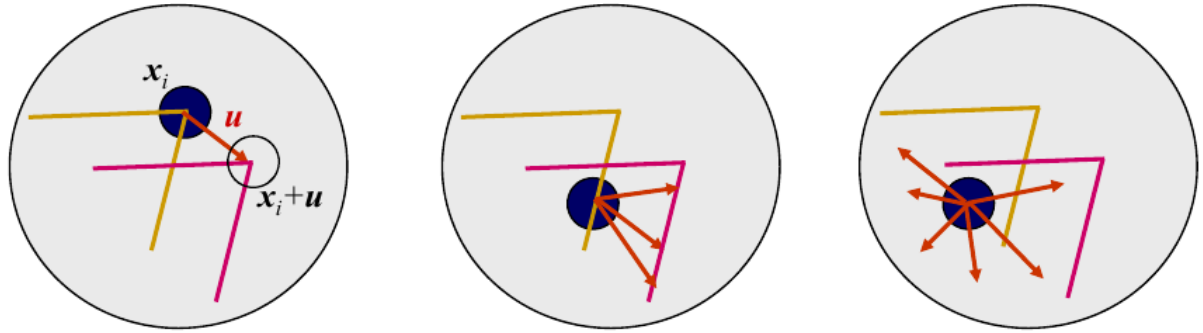
Figure 4: Aperture problem for patches detected from different primitives. Source: Szeliski.
The above figure illustrates the aperture problem. Consider a flat surface without texture. If we generate a patch around any arbitrary point, it will have many correspondences with other patches. It may be obvious that picking any arbitrary point on a flat, single-colored surface would not be descriptive enough to match with anything useful.
What about an edge? An edge is distinct based on its orientation. The middle image in the figure above shows that, while some ambiguity has been resolved, there are still a wide range of possible locations that it could be matched to. There could be many such edges found between images.
This brings us to a corner. A corner has two distinct gradient changes which make it a perfect candidate for interest point detection.
Detecting Corners
Corners are a great choice for a feature. They are small, rotation and translation invariant, and can be computed simply from the gradient images we have computed before.
There are a few distinct interest points of a violin. Maybe we can use a corner detector to come up with patches which can be reproduced across different images.
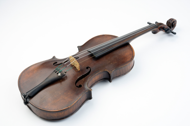
Figure 5: A replica violin.
In a local window, a corner exhibits a large change in orientation. A flat surface has no orientation response at all. An edge only has an orientation in one direction.
How can we detect such changes in an image?
The sum of square differences (SSD). If we take some window and move it over some image, taking a the SSD at each point, we can produce an image of responses. SSD is defined as
\[ f(x, y) = \sum_{(u, v) \in W}\big(I(x + u, y + v) - I(u, v)\big)^2. \]
This Stack Exchange answer provides an excellent visualization of what SSD is achieving here.
This difference was previously used to evaluate discrete steps. Harris et al. note this as a limitation and instead aim to evaluate all possible small shifts about the origin of the shift. Another issue with evaluating SSD as above is efficiency. Iterating and shifting a window over each pixel is extremely inefficient. Through analytic expansion of the term \(I(x + u, y + v)\), we can approximate all possible small shifts around the origin efficiently.
Through Taylor expansion, this can be approximated as
\begin{align*} I(x + u, y + v) &= I(u, v) + x \frac{\partial}{\partial x}I(x, y) + y \frac{\partial}{\partial y}I(x, y) + O(x^2, y^2) \\ &\approx I(u, v) + xI_x + yI_y \end{align*}
In the above approximation, \(O(x^2, y^2)\) describes the upper bound of the behavior of the function. Through Taylor expansion, we could write the higher order terms. However, we only care about small shifts about the shift origin, so only a first order, or linear, approximation is sufficient.
Using this first order approximation, SSD can be written
\begin{align*} f(x, y) &\approx \sum_{(u, v) \in W} w(u, v) \big(I(u, v) + xI_x + yI_y - I(u,v)\big)^2\\ &= \sum_{(u, v) \in W} w(u, v) \big(xI_x + yI_y\big)^2\\ &= \sum_{(u, v) \in W} w(u, v) \big(x^2I_x^2 + 2xyI_xI_y + y^2I_y^2\big) \end{align*}
The term \(x^2I_x^2 + 2xyI_xI_y + y^2I_y^2\) is a linear combination and can be efficiently computed via matrix multiplication.
\begin{equation*} x^2I_x^2 + 2xyI_xI_y + y^2I_y^2 = \begin{bmatrix} x & y \end{bmatrix} \begin{bmatrix} I_x^2 & I_x I_y \\ I_x I_y & I_y^2\\ \end{bmatrix} \begin{bmatrix} x\\ y \end{bmatrix} \end{equation*}
We can now rewrite the original SSD as follows.
\begin{equation*} f(x, y) \approx \begin{bmatrix} x & y \end{bmatrix} M \begin{bmatrix} x\\ y \end{bmatrix}, \end{equation*}
where
\begin{equation*} M = \sum_{(u, v) \in W} w(u, v) H. \end{equation*}
\begin{equation*} H = \begin{bmatrix} I_x^2 & I_x I_y\\ I_x I_y & I_y^2 \\ \end{bmatrix} \end{equation*}
\(M\) is then an autocorrelation matrix. The benefit of this formulation is that \(M\) is a symmetric matrix. If we remember our studies from linear algebra, we remember that there are some very important properties and characteristics of symmetric matrices.
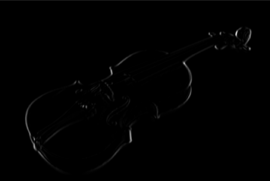
Figure 6: Gradient image (I_x^2).
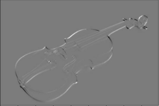
Figure 7: Gradient image (I_x I_y).
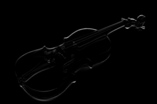
Figure 8: Gradient image (I_y^2).
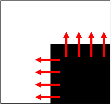
Figure 9: Gradient change in both (x) and (y). Credit: David Jacobs
First, lets consider a simple case of detecting the following corner. At this orientation, the changes in gradient are only in the vertical and horizontal directions. If we consider the matrix \(M\) from above, we would get the following result
\begin{equation*} M = \begin{bmatrix} \sum I_x^2 & \sum I_x I_y\\ \sum I_x I_y & \sum I_y^2 \end{bmatrix} = \begin{bmatrix} \lambda_1 & 0\\ 0 & \lambda_2 \end{bmatrix}. \end{equation*}
The off-diagonal entries will be 0, by definition of the dot product and orthogonal vectors. The entries on the main diagonal will represent the eigenvalues of \(M\). If both entries on the main diagonal are large, this would indicate a large change in orientation within the window.
What if the corner is not as ideal?
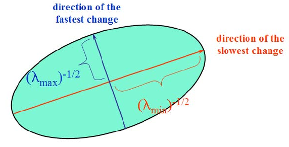
Figure 10: Eigenvalue analysis of autocorrelation matrix. Source: Szeliski.
Relationship to Eigenvalues
Recall the Spectral Theorem for Symmetric Matrices, which states: A symmetric matrix \(A \in \mathbb{R}^{n\times n}\) has the following properties:
- A has \(n\) real eigenvalues, counting multiplicities.
- The dimension of the eigenspace for each eigenvalue \(\lambda\) equals the multiplicity of \(\lambda\) as a root of the characteristic equation.
- The eigenspaces are mutually orthogonal, in the sense that eigenvectors corresponding to different eigenvalues are orthogonal.
- \(A\) is orthogonally diagonalizable.
Symmetric matrices are orthogonally diagonalizable. Thus, a symmetric matrix \(A\) can be written as \(A = PDP^{-1}\), where the columns of \(P\) are the eigenvectors and \(D\) are the corresponding eigenvalues. Another perspective of this is that \(A\) is an ellipse with axis lengths determined by the eigenvalues (diagonal entries of \(D\)) rotated by \(P\).
The eigenvalues of \(M\) can be classified into different regions depending on if they are indicative of a flat region, edge, or corner.
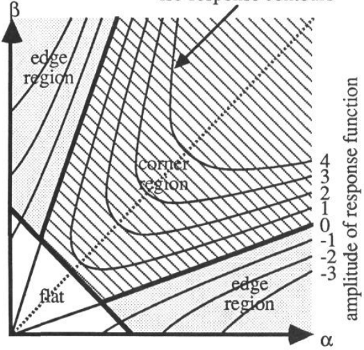
Figure 11: Classification of responses. Source: Harris (1988).
Performing eigendecomposition seems cumbersome in this case. There must be a simpler way we could compute these responses.
We can then approximate this response!
\begin{align*} R &= \det H - \alpha \cdot \textrm{tr}(H)^2\\ &= I_x^2 \cdot I_y^2 - (I_x I_y)^2 - \alpha\big(I_x^2 + I_y^2\big)^2 \end{align*}
If there is a corner, the gradient values will depict orthogonality. That is, the middle term in the equation above will be smaller. This results in a larger response.
The larger the value from the middle term, the less orthogonality is present. This results in a smaller response. In practice, we will see a negative response.
In practice, \(\alpha \in [0.04, 0.06]\).
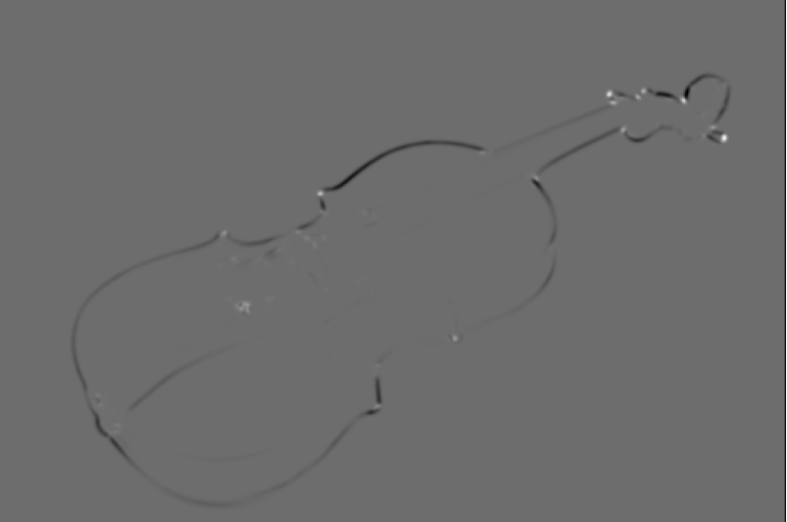
Figure 12: Response image (R).
Window Selection
What is the best window to choose when computing responses across an image? Harris et al. considered this in their original formulation when comparing to Moravec’s corner detection function. Using a flat window with uniform values produces a binary response when over interest points and 0 everywhere else. This can be written as
\begin{equation*} M = \sum_{u, v} w(u, v) \begin{bmatrix} I_x^2 & I_x I_y\\ I_x I_y & I_y^2 \end{bmatrix} \end{equation*}
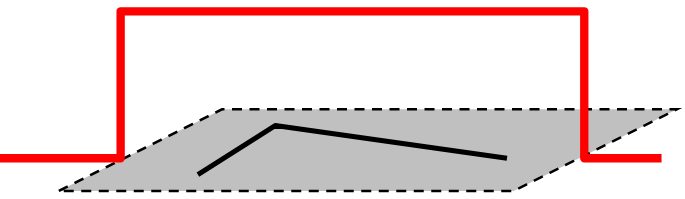
Figure 13: Uniform response window. Results in 1 for interest points inside the window, 0 otherwise. Credit: Fei-Fei Li
Instead, Harris et al. propose using a circular Gaussian window which can be computed as
\begin{equation*} M = g(\sigma) * \begin{bmatrix} I_x^2 & I_x I_y\\ I_x I_y & I_y^2 \end{bmatrix} \end{equation*}
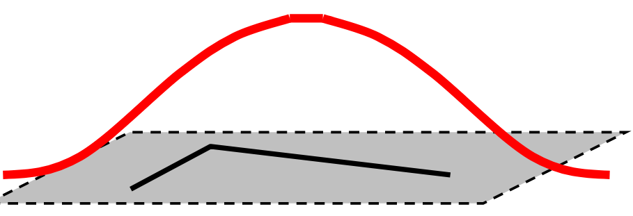
Figure 14: Gaussian window response. Credit: Fei-Fei Li
The Guassian window is easy enough to compute and has the added bonus of making the responses rotation invariant!
Nonmaxima Suppression (Again)
We now have a response image in which each pixel gives an indication as to whether a corner has been detected. To thin out these hypotheses, we will need to suppress neighborhood values that are not maximal. Just like with Edge Detection, we will need to employ nonmaxima suppression.
Before applying that, we may choose to threshold the image to filter out points that are obviously not candidates.
The approach is quite simple here:
- Slide a \(3 \times 3\) window across the image.
- If the center pixel is not the maximum value in the \(3 \times 3\) window, set it to 0.
- Continue until all pixels are evaluated.
Our final result is shown below. The detected corners are marked.

Figure 15: Final output of corner detection.
Describing Image Patches
Given a list of interest points, we can start to build a collection of regions or patches surrounding the point which are useful for feature matching. The simple choice here is to take a fixed size patch surrounding an interest point and use it as a template. We can then compare that to other interest points in different images to see how well they score. There are many limitations to this naive approach that prevent it from working well in general. Even if the perspective of the object is the same in multiple images, slight changes is brightness could affect the matching scores greatly.
Another consideration is scale. If we have an interest point at one scale, will it be detected when that image is scaled by some factor \(k\)?
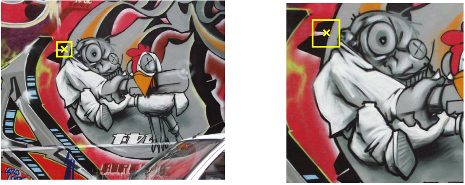
Figure 16: Patch surrounding a similar interest point at different scales. Credit: Kristen Grauman, B. Liebe.
However we choose to represent the information surrounding an interest point need to be robust to translation, scale, and orientation changes. It is important to note that, although the Harris corner detector is invariant to orientation, a naive image patch surrounding the interest point may not be.
Scale Invariance
Is the Harris corner detector scale-invariant?
No! Consider the figure below.
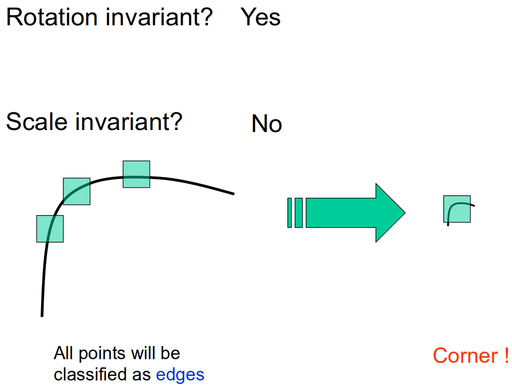
Figure 17: Harris corner detector is not scale invariant. Credit: Kristen Grauman
The output from the detector will be different depending on scale. One solution would be to resize the image over several different scales and consolidate the detections. Doing this would produce many features and take much longer to compute.
Given some feature template that is centered on an interest point, we would expect that size of the patch scales with the scale change of the image itself. This property will drive the development of a scale-invariant method. We select the size of the patch by placing some dark blob with a light background (or vice versa) over the interest point and then selecting the size which provides the greatest response.
Laplacian Filter
A good choice for this is the Laplacian filter. The Laplacian of a 2D function is
\begin{equation*} (\nabla^2 f)(x, y) = \frac{\partial^2 f}{\partial x^2} + \frac{\partial^2 f}{\partial y^2}. \end{equation*}
The Laplacian filter is created following the derivation in the two figures below.
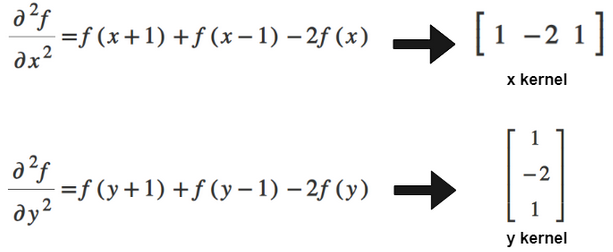
Figure 18: Deriving second partial derivative filters for x and y. Source: https://theailearner.com/2019/05/25/laplacian-of-gaussian-log/
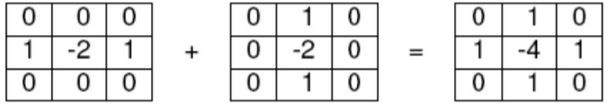
Figure 19: Combining the x and y filters. Source: https://theailearner.com/2019/05/25/laplacian-of-gaussian-log/
It is also common to smooth the operator before use. This can be done by convolving with a Gaussian kernel:
\begin{equation*} K_{\nabla^2} * G_{\sigma}. \end{equation*}
This is referred as the Laplacian of Gaussian filter.
Scale Space
We can use the Laplacian of Gaussian to find the appropriate size of image patch for a given scale. This is achieved by computing a scale-space representation of an image. When we resize an image to make it smaller, there is a loss of information. Similarly, blurring the image causes a loss of information. The larger the \(\sigma\) value for the Gaussian, the more information that is lost. Thus, we can quickly compute different scale-image representations by applying Gaussian blurring with a range of \(\sigma\) values.
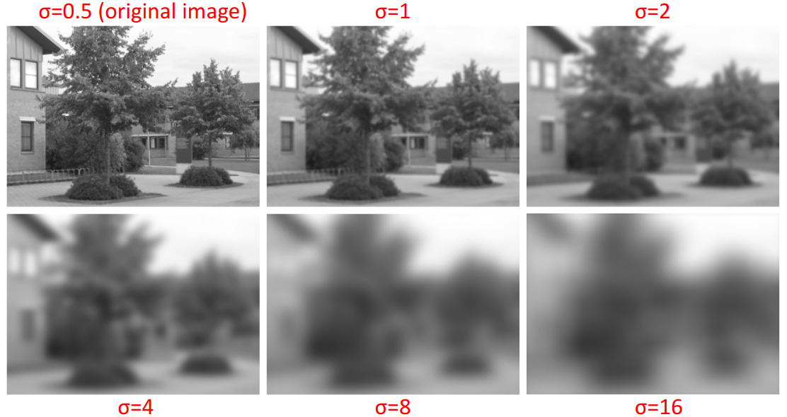
Figure 20: Scale space representations. Source: Wikipedia
As it turns out, blurring and resizing correspond with each other. This is calculated by applying a Gaussian blur to the image following:
\begin{equation*} L_f(\sigma) = f(G_\sigma * I). \end{equation*}
This is the response of function \(f\) in scale-space \(\sigma\).

Figure 21: Selecting features at different scales. Credit: Kristen Grauman
The size of the patch can be found by iterating through different values of \(\sigma\), applying the Laplacian at each scale, and selecting the value of \(\sigma\) which produced the greatest result.
Consider a simple rounded square as depicted below.

Figure 22: Simple rounded square.
If we apply the LoG filter to select the scale which gives the greatest response for the region centered on the top left corner at the original scale, we produce the following graph.
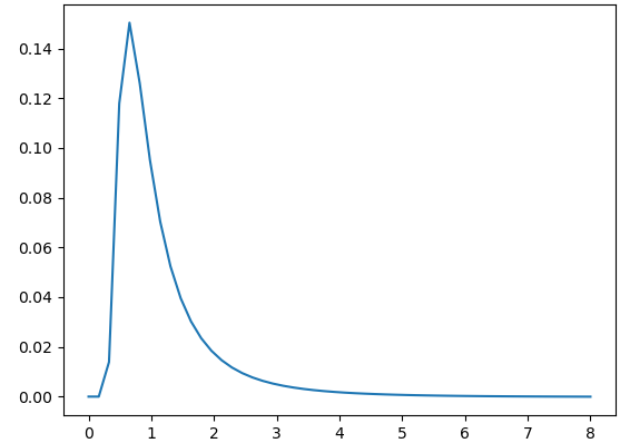
Figure 23: Responses of LoG at the top left corner from (sigma = 0) to (sigma = 8).
If we scale the original image by 2 and apply the same analysis again, we get the following graph.
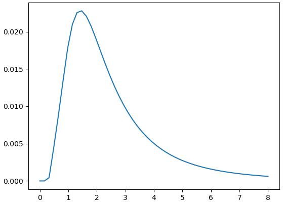
Figure 24: Responses of LoG at original image size at the top left corner from (sigma = 0) to (sigma = 8).
To summarize, using this method will allow us to select the appropriate scale at which our interest point provides the strongest response. However, the cost of this search is high. As we increase the size of the filters, the more work required for each convolution.