Introduction to Data Structures
Introduction to Data Structures
Data structures are fundamental concepts in computer science that allow us to organize and store data in a way that enables efficient access and modification. They are essential building blocks for creating efficient and sophisticated computer programs and databases. Different types of data structures include arrays, linked lists, stacks, queues, trees, graphs, and many more, each serving a specific purpose and suited to specific applications.
Understanding data structures is therefore important because they are used in almost every software application. For instance, social media applications use data structures to store user information and their connections, while search engines use them to index and retrieve web pages quickly. The choice of the right data structure significantly impacts the performance, scalability, and resource utilization of software applications.
Having a strong grasp of data structures and their properties is critical for anyone working with software or data in general. Through studying the benefits and limitations of each data structure, you will be equipped to analyze the efficacy of existing systems as well as make the right choice when developing new ones.
Why Do We Need So Many?
There are many data structures available because no single dataset works best for all cases. Each data structure has its unique characteristics, advantages, and disadvantages. These differences can often be evaluated quantitatively, providing rigorous backing when selecting the appropriate one for the task at hand.
For example, arrays are excellent when the size of the data is known and constant, but they are not efficient when it comes to frequent insertions and deletions. Linked lists, on the other hand, allow for efficient insertions and deletions but are not as quick as arrays when it comes to accessing elements. Trees are invaluable when we need to maintain a sorted list of data and perform quick searches, insertions, and deletions, while hash tables are optimal for scenarios where we need to perform fast lookups.
Review: Pointers
What are Pointers?
Pointers are variables in programming that store the memory address of another variable. They are a powerful feature in many programming languages, including C and C++, allowing programmers to directly access memory locations and manipulate data efficiently. Pointers are crucial for implementing dynamic data structures like linked lists, trees, and graphs.
In Python, pointers are not exposed explicitly as in languages like C, but references, which are similar to pointers, are used to hold the memory address of objects. Understanding the concept of pointers and references is essential for managing memory effectively and avoiding issues like memory leaks and dangling pointers in languages that allow direct memory manipulation. Even if we are not dealing with pointers directly, studying them is beneficial for understanding algorithms and data structures in general.
How are They Represented?
In languages like C, pointers are represented using the asterisk (*) symbol, and the address operator (&) is used to retrieve the memory address of a variable. For example, int *p; declares a pointer to an integer, and p = &x; assigns the address of the variable x to the pointer p.
In Python, pointers are not explicitly represented, but references to objects are used to achieve similar functionality. For instance, when a list is assigned to a new variable, the new variable holds a reference to the same list object, not a copy of the list. Any modifications made through one variable are reflected in the other.
Arrays
How are Arrays Represented in Memory?
Arrays are fundamental data structures that store elements of the same type in contiguous memory locations. The elements can be accessed randomly by indexing into the array. In memory, an array is represented as a block of memory cells, each holding an element of the array placed side by side. The size of each cell is determined by the size of the array’s element type.
The base address of the array is the memory address of the first element (index 0), and it is used, along with the index and the size of each element, to calculate the address of any element in the array. For example, if the base address is `B`, the size of each element is `S`, and the index of the element is `i`, the address of the element can be calculated as `B + (i * S)`.
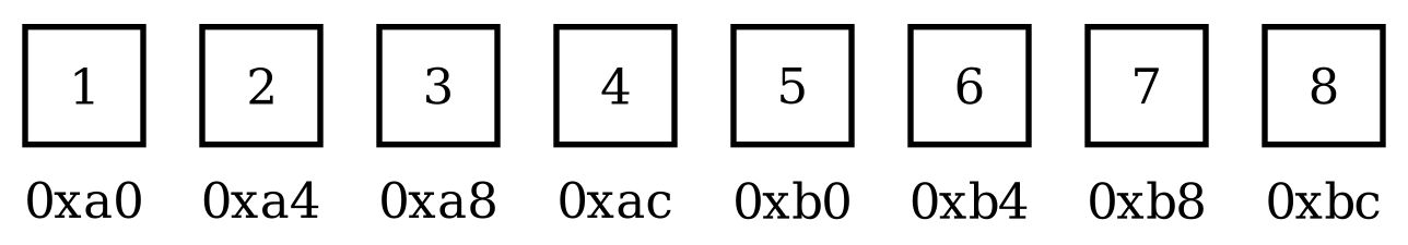
Figure 1: Memory layout of an integer array of size 8.
How Many Bytes Does Each Element Use?
The number of bytes used by each element in an array depends on the data type of the elements. For example, in most systems, an int uses 4 bytes, a char uses 1 byte, and a double uses 8 bytes. When an array is declared, the total memory allocated for the array is the product of the number of elements and the size of each element.
In Python, the sys module can be used to find the size of an object in bytes. However, Python’s dynamic typing and object-oriented nature mean that the size of an array element can vary significantly, as each element is an object that can have additional overhead and can hold references to other objects.
Since Python does not expose pointers explicitly, we can safely program efficient programs without worrying about making common mistakes related to pointers and memory management.
How are Arrays Indexed?
Arrays are indexed using a zero-based indexing system, where the first element is accessed using index 0, the second element with index 1, and so on. To access an element at a specific index, the address of the element is calculated using the base address of the array, the size of each element, and the index of the element.
In languages that support pointers, the address of an element in an array can be calculated using pointer arithmetic. If p is a pointer to the base address of the array, and i is the index of the element, the address of the element can be calculated as p + i, where i is automatically scaled by the size of the array’s element type.
Matrices
Fixed-sized Arrays vs. Ragged Arrays
Matrices are two-dimensional arrays that can be represented using fixed-sized arrays or ragged arrays. A fixed-sized array is a regular matrix where each row has the same number of columns, and it is represented in memory as a contiguous block. It allows for efficient access to elements using row and column indices but can waste memory if the matrix is sparse.
A ragged array, on the other hand, is an irregular matrix where each row can have a different number of columns. It is represented using an array of pointers, where each pointer points to a one-dimensional array representing a row of the matrix. Ragged arrays are more memory-efficient for sparse matrices but can be more complex to manage and traverse.
Choosing between fixed-sized and ragged arrays depends on the requirements of the application, the characteristics of the matrix, and the trade-offs between memory efficiency and complexity. Understanding the differences between the two representations is crucial for implementing matrices effectively and optimizing memory usage.
Flat Indexing, Back and Forth
Flat indexing is a technique used to represent a two-dimensional array or matrix using a one-dimensional array. In this representation, the elements of the matrix are stored in a single array in row-major or column-major order, and the two-dimensional indices (row and column) are mapped to a single index in the one-dimensional array.
For a matrix with M rows and N columns, the mapping from two-dimensional indices to a one-dimensional index in row-major order is done using the formula index = (row * N) + column, and in column-major order using the formula index = (column * M) + row. Flat indexing allows for efficient memory utilization and easy serialization of matrices but requires conversion between one-dimensional and two-dimensional indices.
Python Example of Matrices
In Python, matrices can be represented using lists of lists, where each inner list represents a row of the matrix. Elements can be accessed and modified using two indices, one for the row and one for the column. For example, to create a 2x3 matrix and access the element in the second row and third column, you can do the following:
matrix = [[1, 2, 3], [4, 5, 6]]
element = matrix[1][2]  # access value 6
NumPy also provides support for multi-dimensional arrays and matrices along with a host of functions to perform operations on them. Using Numpy, you can create a matrix and access its elements as follows:
import numpy as np
matrix = np.array([[1, 2, 3], [4, 5, 6]])
element = matrix[1, 2]  # access value 6
Multi-Dimensional Arrays
Introduction to Multi-Dimensional Arrays
Multi-dimensional arrays are arrays of more than 1 dimension. They are used to represent complex data structures like matrices, tensors, and tables. They are crucial for various applications, including scientific computing, image processing, and machine learning, where data is often multi-dimensional.
In a multi-dimensional array, each element is identified by multiple indices, one for each dimension of the array. For example, in a two-dimensional array representing a matrix, each element is identified by two indices representing the row and column of the element. The number of dimensions and the size of each dimension determine the structure and capacity of the array.
Different languages have different approaches to handling multi-dimensional arrays. C, for example, arranges the memory of any array contiguously. Java and Python use jagged arrays, where the row lengths can differ in size. The data in each row might be contiguous, but the entire array is not.
NumPy Arrays and Their Representation
A NumPy array is represented in memory as a contiguous block, and it allows for efficient access and manipulation of elements using multiple indices. The shape of the array, represented as a tuple of integers, determines the number of dimensions and the size of each dimension of the array.
To determine how to index the contiguous stream of values represented as an $n$-dimensional array, each np.array specifies the strides for each dimension. Consider the following array with shape (2, 3, 4) and data type int32:
import numpy as np
x = np.array([[[1, 2, 3, 4],
               [5, 6, 7, 8],
               [9, 10, 11, 12]],
              [[13, 14, 15, 16],
               [17, 18, 19, 20],
               [21, 22, 23, 24]]], dtype=np.int32)
The strides of the array are (48, 16, 4), which means that to move to the next depth, we need to move 48 bytes, to move to the next row, we need to move 16 bytes, and to move to the next column, we need to move 4 bytes. The strides are calculated based on the size of each element and the shape of the array.
Python Example with NumPy
Here’s an example of how to create a two-dimensional array (matrix) using Numpy and how to access its elements:
import numpy as np
# Creating a 2x3 Numpy array
array = np.array([[1, 2, 3], [4, 5, 6]])
# Accessing the element in the second row and third column
element = array[1, 2]  # element will be 6
NumPy also provides various functions to perform operations on arrays, such as reshaping, transposing, and aggregating. For example, to calculate the sum of all elements in the array, you can use the np.sum function:
total = np.sum(array) # total will be 21
Stacks
How are Stacks Represented with an Array?
A stack is a linear data structure that follows the Last In First Out (LIFO) principle, meaning the last element added to the stack is the first one to be removed. Stacks can be easily implemented using arrays, where elements are added and removed from one end of the array, known as the top of the stack.
When representing a stack with an array, one must keep track of the index of the top of the stack. Elements are added to the stack by placing them at the position indicated by the top index and then incrementing the top index. Elements are removed from the stack by decrementing the top index and then accessing the element at that position.
Difference Between Using the Beginning or the End of the Array as the Top
When implementing a stack using an array, one can choose to use either the beginning or the end of the array as the top of the stack. The choice affects the implementation of the push and pop operations and the way the top index is managed.
If the beginning of the array is used as the top, elements are added and removed from the first position of the array, and the other elements must be shifted to make room or fill the gap. This can lead to higher time complexity for push and pop operations. If the end of the array is used as the top, elements are added and removed from the last position of the array, allowing for constant-time push and pop operations without the need to shift other elements.
Python Example of Stack with Array
Here’s an example of how to implement a stack using a Python list, with the end of the list as the top of the stack:
stack = []  # Initializing an empty stack
stack.append(1)  # Pushing an element onto the stack
stack.append(2)  # Pushing another element onto the stack
top_element = stack.pop()  # Popping the top element from the stack, top_element will be 2
This implementation allows for efficient and simple push and pop operations, with constant time complexity. However, the size of the stack is limited by the available memory, and care must be taken to handle underflow and overflow conditions.
Understanding how to implement and use stacks is crucial for solving problems that involve reversing, balancing, or processing data in a LIFO manner. Stacks are a versatile and fundamental data structure used in various applications, including expression evaluation, syntax parsing, and undo mechanisms.
Queues
How are Queues Represented with an Array?
A queue is a linear data structure that follows the First In First Out (FIFO) principle, meaning the first element added to the queue is the first one to be removed. Queues can be implemented using arrays, where elements are added at the rear and removed from the front.
When representing a queue with an array, two indices are maintained, one for the front and one for the rear of the queue. Elements are enqueued by placing them at the position indicated by the rear index and then incrementing the rear index. Elements are dequeued by accessing the element at the front index and then incrementing the front index.
Downside to Using One Side of the Array as the Front and the Other as the Rear
When implementing a queue using an array, using one side of the array as the front and the other as the rear can lead to inefficient use of space. Once elements are dequeued from the front, the space they occupied cannot be reused, and overflow can occur even if there is free space at the front of the array.
To overcome this limitation, a circular queue can be implemented, where the front and rear indices wrap around to the beginning of the array when they reach the end. This allows for efficient use of space and avoids overflow as long as there is free space in the array. However, it requires more complex index management and can be harder to implement correctly.
More Efficient Approach by Using a Reference to a Head and Tail
A more efficient approach to implementing a queue is to use a linked list, where each element holds a reference to the next element in the queue. This allows for dynamic resizing of the queue and efficient enqueue and dequeue operations, without the need for complex index management or wasted space.
In this approach, two pointers are maintained, one for the head (front) and one for the tail (rear) of the queue. Elements are enqueued by adding them at the position pointed to by the tail pointer and updating the tail pointer to the new element. Elements are dequeued by accessing the element pointed to by the head pointer and updating the head pointer to the next element.
This same approach can be done by using indices for the head and tail. The data itself is “circular” in the sense that the indices wrap around to the beginning of the array when they reach the end. This allows for efficient use of space and avoids overflow as long as there is free space in the array.
Python Example of a Queue using an Array
Here’s an example of how to implement a simple queue using a Python list, with the front at the beginning of the list and the rear at the end of the list:
from collections import deque
queue = deque()  # Initializing an empty queue
queue.append(1)  # Enqueueing an element
queue.append(2)  # Enqueueing another element
front_element = queue.popleft()  # Dequeueing the front element from the queue, front_element will be 1
This implementation uses the deque class from the collections module, which allows for efficient appending and popping from both ends of the list. It provides a simple and versatile way to implement a queue in Python, with dynamic resizing and constant-time enqueue and dequeue operations.
Understanding how to implement and use queues is essential for solving problems that involve processing data in a FIFO manner. Queues are a fundamental and versatile data structure used in various applications, including task scheduling, order processing, and breadth-first search.