Introduction to GPGPU Programming
Structure of the Course
The primary of this goal is of course to learn how to program GPUs. A key skill that will be developed is the ability to think in parallel. We will start with simple problems that are embarrassingly parallel and then move on to more complex problems that require synchronization. One of the biggest challenges will be in converting processes that are simple to reason about in serial to parallel processes.
The course is divided into three parts. The first part will cover the fundamentals of heterogeneous parallel computing and the CUDA programming model. We will focus on problems that are mostly embarrassingly parallel, but will also step into more complicated problems.
The second part will cover primitive parallel patterns. These are patterns from well-known algorithms that can be used to solve a wide variety of problems. Think of these as useful blueprints for solving problems in parallel. During the second part, we will also dive into more advanced usages of CUDA.
Part three will cover advanced patterns from more specific applications, such as iterative MRI reconstruction. The course will conclude with expert practices.
There will be regular assignments that focus on the concepts learned throughout the course. These will typically be accompanied by a series of questions to reinforce and verify that you are successful in each step. Quizzes will be given after each assignment to serve as a checkpoint.
Heterogeneous Parallel Computing
Heterogeneous computing refers to systems that use more than one kind of processor or core. One common theme in the course will be to focus on a perfect union between the CPU and GPU. Not every task can be fully parallelized. Many tasks are well suited for sequential processing and others are better suited for parallel processing. Parallelism can be further broken down into data parallelism and task parallelism. The majority of our time will be focused on data parallelism, but it is important to keep in mind that not everything fits into this category. Over time, you will develop a sense for what fits this paradigm and what does not.
The idea of parallelism is certainly not new, but it has become ubiquitous in the computing space. Consider 30 years ago, when most consumer computers had a single core. The race between chip designers resulted in increasing single-core performance year after year in the form of increased clock speeds. This was a great way to increase performance, but it came at the cost of increased power consumption and heat. Scaling down transistors has also be a tried and true way of decreasing processor size and increasing performance. However, we are quickly reaching a physical limit on the size of a transistor.
The solution to these problems is the same solution seen in scaling up large systems: horizontal scaling. The intuition is straightforward: many things can do the work faster than a single thing. For large-scale systems, the answer is distributed systems in which no single unit needs to be overly powerful or complicated. For consumer processors, this comes in the form of additional cores on a chip.
In the context of CPUs, adding multiple cores means that we have a multi-core homogeneous system. These are general-purpose processors that can complete any computational task. The cores are identical and can be used interchangeably. The cores are also tightly coupled, meaning that they share memory and can communicate with each other. A similar statement can be made for GPUs. Let’s take a look at the differences between them.
Latency vs. Throughput
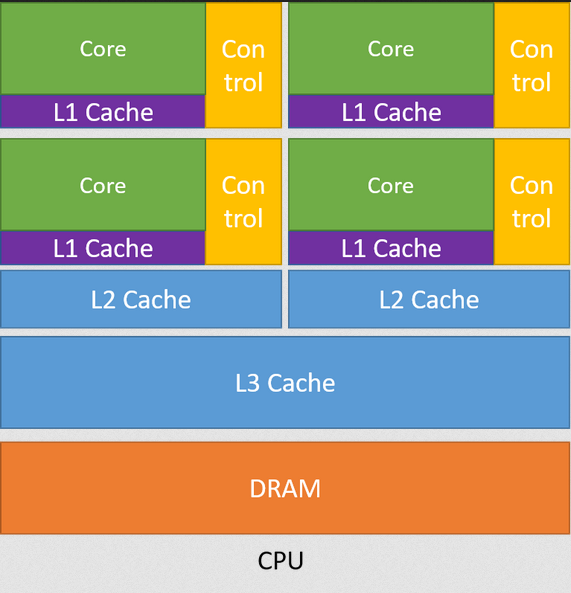
CPUs follow a latency-first design. The space on the chip itself is not fully dedicated to the processing units. Instead, space is reserved for things like cache, branch prediction, and other features that reduce latency. All computational tasks can be completed on a CPU, but the throughput may be lower than a GPU.
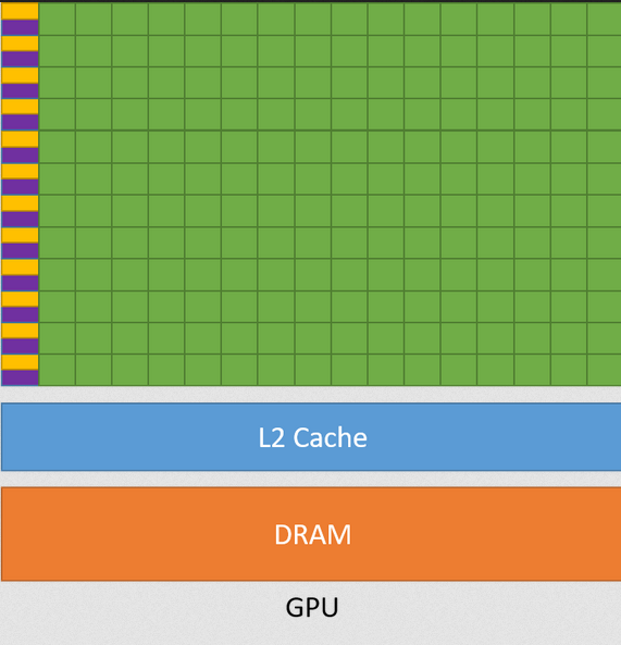
GPUs follow a throughput-first design. The space on the chip is dedicated to processing units such as ALUs. The cores themselves are not as sophisticated as those found on a CPU. Communication between cores takes more time and is more difficult, but having more of them means that the raw throughput of the chip is higher.
The development of GPUs was driven by the gaming industry, specifically with rendering, where many vertices and pixels need to be processed in parallel. As we explore GPU solutions to different problems, we will see that data delivery is a key bottleneck. There are techniques available to get around this, which we will need to study closely.
GPUs and Supercomputing
GPUs are featured in many of the top 500 supercomputers. This goes to show that they are a powerful and cost-efficient tool for solving problems. The table below shows the top 5 supercomputers as of November 2023. 4 of them utilize some form of GPU acceleration.
| Name | CPUs | GPUs | Peak PFlop/s |
|---|---|---|---|
| Frontier (Oak Ridge NL) | 606,208 cores | 37,888 AMD MI250X | 1,679.72 |
| Aurora (Argonne NL) | 1,100,000 cores (est.) | 63,744 Intel GPU Max | 1,059.33 |
| Eagle (Microsoft Azure) | 1,123,200 cores (combined) | Unknown Split (NVIDIA H100) | 846.74 |
| Fugaku | 7,630,848 cores | None | 537.21 |
| LUMI | 362,496 cores | 11,712 AMD MI250X | 531.51 |
The results are clear: heterogeneous parallel computing is a powerful tool for solving problems. Learning how to use these tools will be a valuable skill for the future.
Measuring Speedup
In general, if system A takes \(T_A\) time to complete a task and system B takes \(T_B\) time to complete the same task, then the speedup of system B over system A is given by \(S = \frac{T_A}{T_B}\).
Amdahl’s law is defined as follows:
\[S(s) = \frac{1}{(1 - p) + \frac{p}{s}}\]
where \(p\) is the fraction of the task that can be parallelized and \(s\) is the speedup of the part of the task that can be parallelized.
It is not common that 100% of a task can be parallelized. Amdah’s law takes this into account. Suppose that 40% of a given task can benefit from parallelization. If that part of the task can be sped up by a factor of 10, then the overall speedup is given by:
\[S = \frac{1}{(1 - 0.4) + \frac{0.4}{10}} = 1.56\]
In virtually every lab that you will do in this course, you will be asked to measure the speedup of your solution. This is a good way to verify that your solution is correct and that it is actually faster than the serial version. This will also be a critical part of your project, where you will first need to create a serial version of your solution and then parallelize it.
GPU Programming History
Early GPU programming was done using OpenGL and DirectX. These were graphics APIs, so everything had to be done in terms of pixel shaders. Researchers found ways to use these APIs to do general purpose computing, but it was very difficult since one could not easily debug the code. Essentially, the input had to be encoded as a texture or color. The GPU would then process the texture and output the result as a texture. The output would then have to be decoded to get the result.
In 2006, NVIDIA unveiled the GeForce 8800 GTX, which was the first DirectX 10 GPU. More importantly, it was the first GPU built using the CUDA architecture. CUDA also refers to the programming model that NVIDIA developed to facilitate general purpose GPU programming. A key piece of the CUDA architecture is the unified shader pipepline, which allows each ALU to be utilized for general purpose computations.
The different ALUs have access to a global memory space as well as a shared memory space managed by software. We will explore the specifics of this architecture in part 1 of this course. Since that time, many major changes have been made to the CUDA architecture. Additionally, many other standards have been developed to facilitate GPU programming and parallel computing in general.
One of the most important standards, which we also study in this course, is OpenCL. OpenCL is an open standard that allows for heterogeneous parallel computing. It is supported by many different vendors, including NVIDIA, AMD, and Intel. OpenCL is a C-like language that allows for the creation of kernels that can be executed on a variety of devices. The OpenCL standard is maintained by the Khronos Group, which also maintains the OpenGL standard.
Applications
We are currently in the midst of a data explosion. Vertical scaling, the idea of improving a single system, cannot meet the demands of modern challenges. Horizontal scaling is the most sure solution for now. Distributed systems utilize cheap, commodity servers in lieu of complex supercomputers to distribute applications to mass markets. Parallel computation has applications in just about every field imaginable. We will try to cover a wide variety of applications, as many of them feature parallel solutions that are helpful in other domains.
Linear Algebra Libraries
One of the most widely utilized applications of data parallelism is in linear algebra libraries. Common matrix operations such as matrix multiplication and matrix inversion are highly parallelizable. The cuBLAS library is a highly optimized implementation of these operations.
For a great overview of the evolution of linear algebra libraries and the impact of GPUs, see Jack Dongarra’s keynote speech at the 50 Years of Computing at UTA event.
Machine Learning
Model training and optimization in machine learning is a perfect candidate for data parallelism. Large models such as Llama2 require a massive amount of data to train (Touvron et al. 2023). Deep learning models such as this are trained on many GPUs that can execute functions on independent data points in parallel.
NVIDIA has developed a useful library, which we will study in this course, called cuDNN that implements highly optimized implementations of common functions used in a deep learning pipeline. High level frameworks build off of this library to provide easier development interfaces for machine learning practitioners. Popular examples include PyTorch, TensorFlow, and JAX.
Computer Vision
Most of the current state-of-the-art computer vision methods are driven by deep learning, so they also benefit greatly from data parallelism. Convolutional Neural Networks (CNN) have been the driving force behind machine-learning based computer vision methods. They are parameter efficient and take advantage of data parallelism. We will study the core operation behind this model, the convolutional opreator.

Figure 3: 2D Convolution on a 4x4 grid using a 3x3 filter with unit stride (Dumoulin and Visin 2018)
Computational Chemistry
CUDA has been utilized for computing heat transfer calculations efficiently (Sosutha and Mohana 2015). The authors found that the computations could be computed independently, which is perfect for a parallel architecture like a GPU, where throughput is preferred to latency.
Other Applications
There are many other applications of data parallelism, some of which we will explore and learn from in this course. Examples include the following.
- Financial Analysis
- Scientific Simulation
- Engineering Simulation
- Data Intensive Analytics
- Medical Imaging
- Digital Audio Processing
- Digital Video Processing
- Biomedical Informatics
- Electronic Design Automation
- Statistical Modeling
- Numerical Methods
- Ray Tracing Rendering
- Interactive Physics
What to expect from this course
This course is extremely hands-on. Almost every topic we cover will have an associated programming exercise. Some of these exercises will be integrated into assignments, other will be presented as in-class demonstrations. The fact that there are so many applications means you will need to be able to adapt to new domains quickly. By the end of this course, you should have acquired the following skills:
- Advanced familiarity with the CUDA programming model
- Ability to think in parallel
- Identify sections of code that can be parallelized
- Implementation of parallel solutions
- Debugging parallel code
- Measuring performance increase from parallelization

