Introduction to Graph Theory
What are Graphs?
A graph is a data structure that is used to represent pairwise relationships between objects. Graphs are used in many applications, such as social networks, maps, and routing algorithms. These notes accompany the series of lectures on graphs for my Foundations of Computing course at the University of Texas - Arlington.
Definitions
-
A directed graph \(G\) is represented as a pair \((V, E)\) of a set of vertices \(V\) and edges \(E\). Edges are represented as ordered pairs.
-
An undirected graph \(G\) is represented as a pair \((V, E)\) of a set of vertices \(V\) and edges \(E\). The edges are represented as unordered pairs, as it does not matter which direction the edge is going.
-
Let \((u, v)\) be an edge in a graph \(G\). If \(G\) is a directed graph, then the edge is incident from \(u\) and is incident to \(v\). In this case, \(v\) is also adjacent to \(u\). If \(G\) is an undirected graph, then the edge is incident on \(u\) and \(v\). For undirected graphs, the adjacency relation is symmetric.
-
The degree is a graph is the number of edges incident on a vertex. For directed graphs, the in-degree is the number of edges incident to a vertex, and the out-degree is the number of edges incident from a vertex.
-
A path from a vertex \(u\) to another vertex \(v\) is a sequence of edges that starts at \(u\) and ends at \(v\). This definition can include duplicates. A simple path is a path that does not repeat any vertices. A cycle is a path that starts and ends at the same vertex. If a path exists from \(u\) to \(v\), then \(u\) is reachable from \(v\).
-
A connected graph is a graph where there is a path between every pair of vertices. A strongly connected graph is a directed graph where there is a path between every pair of vertices. The connected components of a graph are the subgraphs in which each pair of nodes is connected by a path. In image processing, connected-component labeling is used to find regions of connected pixels in a binary image.
-
Let \(G = (V, E)\) and \(G’ = (V’, E’)\). \(G\) and \(G’\) are isomorphic if there is a bijection between their vertices such that \((u, v) \in E\) if and only if \((f(u), f(v)) \in E’\).
-
A complete graph is an undirected graph in which every pair of vertices is adjacent. A bipartite graph is an undirected graph in which the vertices can be partitioned into two sets such that every edge connects a vertex in one set to a vertex in the other set.
-
A multi-graph is a graph that allows multiple edges between the same pair of vertices. These are commonly in social network analysis, where multiple edges between two people can represent different types of relationships.
TODO: Add figures demonstrating the above definitions
Representations
Graphs can be represented in many different ways. The most common representations are adjacency lists and adjacency matrices. Adjacency lists are more space-efficient for sparse graphs, while adjacency matrices are more space-efficient for dense graphs. Adjacency lists are also more efficient for finding the neighbors of a vertex, while adjacency matrices are more efficient for checking if an edge exists between two vertices.
Example: Adjacency Matrix and Reachability
Consider the graph in the figure below.
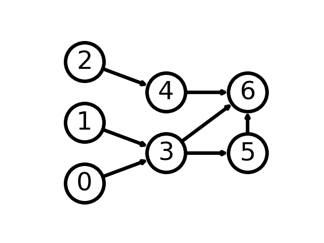
Figure 1: A directed graph
The adjacency matrix for this graph is:
\begin{bmatrix} 0 & 0 & 0 & 1 & 0 & 0 & 0\\ 0 & 0 & 0 & 1 & 0 & 0 & 0\\ 0 & 0 & 0 & 0 & 1 & 0 & 0\\ 0 & 0 & 0 & 0 & 0 & 1 & 1\\ 0 & 0 & 0 & 0 & 0 & 0 & 1\\ 0 & 0 & 0 & 0 & 0 & 0 & 1\\ 0 & 0 & 0 & 0 & 0 & 0 & 0\\ \end{bmatrix}
The rows and columns represent the vertices in the graph. The value at row \(i\) and column \(j\) is 1 if there is an edge from vertex \(i\) to vertex \(j\). Otherwise, the value is 0. Let \(A\) be the adjacency matrix for a graph \(G\). The matrix \(A^k\) represents the number of paths of length \(k\) between each pair of vertices. For example, \(A^2\) for the above graph is:
\begin{bmatrix} 0 & 0 & 0 & 0 & 0 & 1 & 1\\ 0 & 0 & 0 & 0 & 0 & 1 & 1\\ 0 & 0 & 0 & 0 & 0 & 0 & 1\\ 0 & 0 & 0 & 0 & 0 & 0 & 1\\ 0 & 0 & 0 & 0 & 0 & 0 & 0\\ 0 & 0 & 0 & 0 & 0 & 0 & 0\\ 0 & 0 & 0 & 0 & 0 & 0 & 0\\ \end{bmatrix}
The value at row \(i\) and column \(j\) is the number of paths of length 2 from vertex \(i\) to vertex \(j\). For example, is a path from vertex 0 to vertex 6 via 0 -> 3 -> 6.
Graph Traversal Algorithms
Graph traversal algorithms are used to explore the structure of a graph. You might initially find this a useless endeavour. If we have defined our own graph, what about it would we need to explore? In scenarios with highly complex and large datasets, the search takes on slightly different meanings. Perhaps we are searching for specific trends based on a range of values such as the Bacon number of a particular celebrity.
Breadth First Search
Breadth First search explores the graph broadly, ensuring one level has been exhausted before moving onto the next. We previously studied breadth-first search in the context of binary search trees. The algorithm is the same when applied on general graphs, but our perspective is slightly different now. The function studied before did not use node coloring. Let’s investigate the algorithm given by Cormen et al. in Introduction to Algorithms (Cormen et al. 2022).
The algorithm adds a color to each node to keep track of its state. The colors are:
- WHITE: The node has not been discovered yet.
- GRAY: The node has been discovered, but not all of its neighbors have been discovered.
- BLACK: The node has been discovered, and all of its neighbors have been discovered.
First, every vertex is painted white and the distance is set to \(\infty\). The first node s is immediately set to have 0 distance. The queue then starts with s. While there are any grey vertices, dequeue the next available node and add its adjacent vertices to the queue. The distance of each adjacent vertex is set to the distance of the current vertex plus one. Once all of its neighbors have been discovered, the current vertex is painted black.
The algorithm and an example run from Cormen et al. are shown below.
def bfs(G, s):
    for u in G.V:
        u.color = WHITE
        u.d = inf
        u.pi = None
    s.color = GRAY
    s.d = 0
    s.pi = None
    Q = Queue()
    Q.enqueue(s)
    while not Q.empty():
        u = Q.dequeue()
        for v in G.adj[u]:
            if v.color == WHITE:
                v.color = GRAY
                v.d = u.d + 1
                v.pi = u
                Q.enqueue(v)
        u.color = BLACK
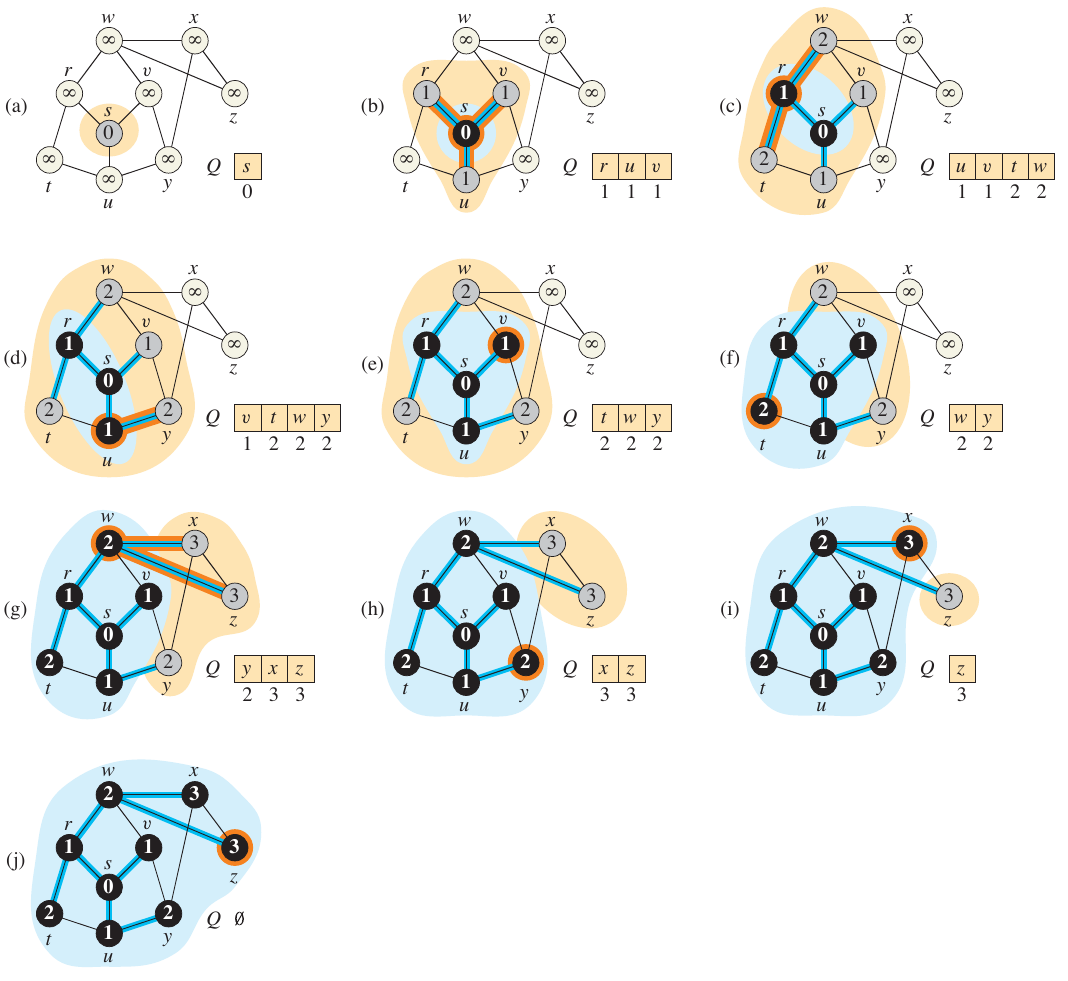
Figure 2: Breadth First Search from Cormen et al.
Analysis
The running time of BFS is \(O(V + E)\), where \(V\) is the number of vertices and \(E\) is the number of edges. Each vertex is queued and dequeued once, so the queue operations take \(O(V)\) time. Each edge is examined once, so the edge operations take \(O(E)\) time. The total running time is \(O(V + E)\).
Breath-first Trees
The blue lines in the previous example depict a breadth-first tree which was built by BFS. The tree is defined by the \(\pi\) values updated throughout the course of the algorithm. These can also be used to reconstruct the shortest path from \(s\) to any other vertex \(v\).
A predecessor subgraph is a graph \(G_{\pi} = (V_{\pi}, E_{\pi})\), where
\begin{align*} V_{\pi} &= \{v \in V : v.\pi \neq \text{None}\} \cup \{s\} \text{ and}\\ E_{\pi} &= \{(v.\pi, v) : v \in V_{\pi} - \{s\}\}. \end{align*}
Such a graph is a breadth-first tree if \(V_{\pi}\) consists of the vertices reachable from \(s\) and, for all \(v \in V_{\pi}\), the subgraph \(G_{\pi}\) contains a unique simple path from \(s\) to \(v\) that is also a shortest path from \(s\) to \(v\) in \(G\).
To print the vertices on a shortest path from \(s\) to \(v\):
def print_path(G, s, v):
    if v == s:
        print(s)
    elif v.pi == None:
        print("No path from", s, "to", v, "exists.")
    else:
        print_path(G, s, v.pi)
        print(v)
Exercise
Run BFS on the following graph, starting from \(s\).
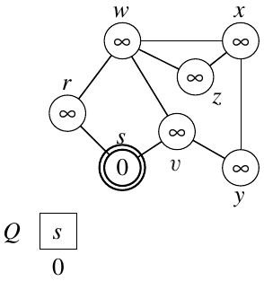
Figure 3: Graph for BFS exercise from Cormen et al.
Depth First Search
Like the BFS algorithm presented in Introduction to Algorithms by Cormen et al., the DFS algorithm also uses colors to keep track of the state of each node. The colors are similar to the BFS algorithm, but the meaning is slightly different:
- WHITE: The node has not been discovered yet.
- GRAY: The node has been visited for the first time.
- BLACK: The adjacency list of the node has been examined completely.
First, all vertices are colored white. The time is set to 0. The function dfs_visit is called on each vertex. The function is defined as follows:
def dfs(G):
    for u in G.V:
        u.color = WHITE
        u.pi = None
    time = 0
    for u in G.V:
        if u.color == WHITE:
            dfs_visit(G, u)

def dfs_visit(G, u):
    time += 1
    u.d = time
    u.color = GRAY
    for v in G.adj[u]:
        if v.color == WHITE:
            v.pi = u
            dfs_visit(G, v)
    u.color = BLACK
    time += 1
    u.f = time
When a node is discovered via dfs_visit, the time is recorded and the color is changed to gray. The start and finish times are useful in understanding the structure of the graph. After all of the node’s neighbors have been discovered, the color is changed to black and the finish time is recorded. That is, the depth from the current node must be fully explored before it is considered finished. The figure below shows the progress of DFS on a directed graph.
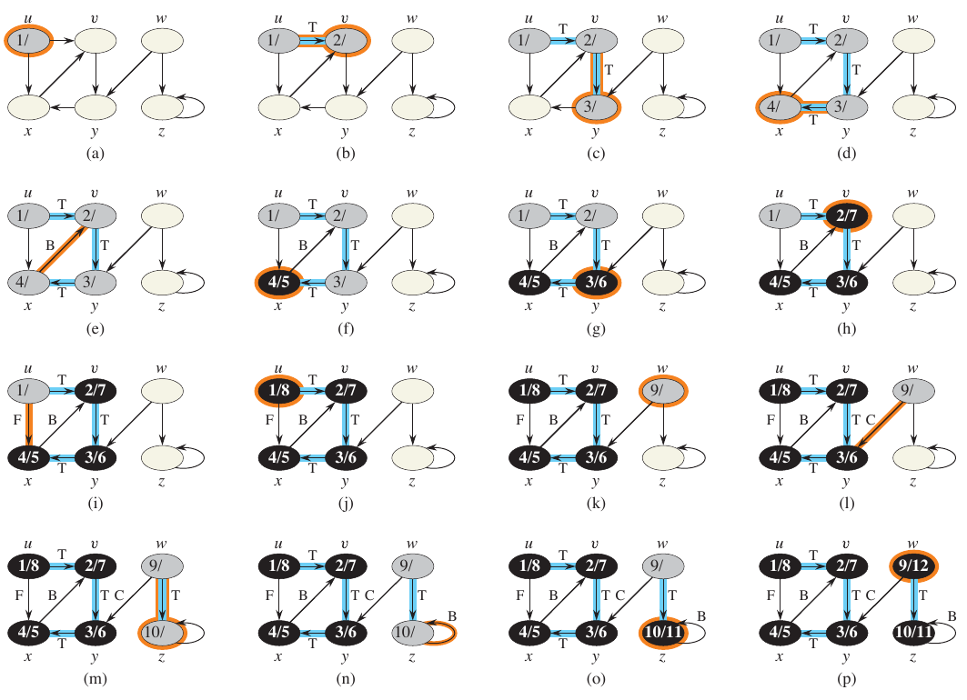
Figure 4: Depth First Search from Cormen et al.
Analysis
Each vertex is added and removed to the queue once. Since these operations are performed in \(O(1)\) time, the total time for these operations in \(O(V)\). When a vertex is dequeued, its adjacency list is scanned. The total number of entries in all adjacency lists is equal to the number of edges, so the time spent scanning these lists of \(O(V + E)\). In summary, the operation is linear in terms of the adjacency-list representation.
Properties of DFS
The predecessor subgraph \(G_{\pi}\) is a forest of trees. That is, it creates a collection of depth first trees.
- What is a forest?
- How does DFS generate a forest?
A vertex \(u = v.{\pi}\) if and only if \(\text{DFS-VISIT}(G, v)\) was called during a search of \(u\)’s adjacency list. Vertex \(v\) is a descendant of vertex \(u\) in the depth-first forest if and only if \(v\) is discovered during the time in which \(u\) is gray (Cormen et al. 2022).
Essentially, each call to dfs_visit from dfs finds a new tree. Let’s consider this on the example above.
Exercise: Draw the DFS forest using the graph above.
Parenthesis Theorem
In a DFS, the discovery and finish times have parenthesis structure. For all \(u, v\), exactly only of the following holds:
- the intervals \([u.d, u.f]\) and \([v.d, v.f]\) are entirely disjoint and neither \(u\) nor \(v\) is a descendant of the other in the depth-first forest.
- the interval \([u.d, u.f]\) is entirely contained within the interval \([v.d, v.f]\) and \(u\) is a descendant of \(v\) in the depth-first forest.
- the interval \([v.d, v.f]\) is entirely contained within the interval \([u.d, u.f]\) and \(v\) is a descendant of \(u\) in the depth-first forest.
It is called the parenthesis theorem because if dfs_visit printed “\((u\)” when it first encountered \(u\) and printed “\(u)\)” when it finished, the expression would be well formed.
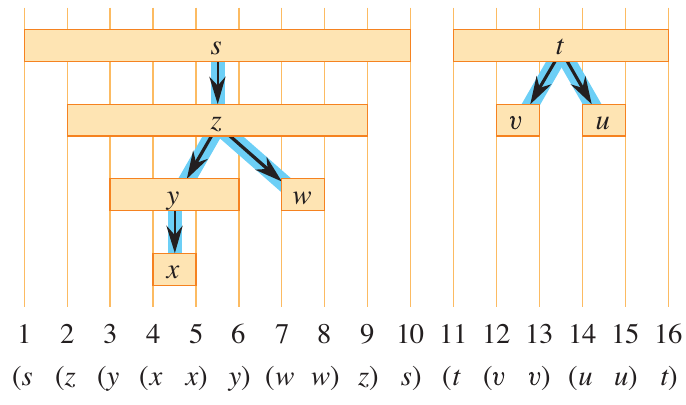
Figure 5: Example of parenthesis structure from Cormen et al.
White-path Theorem
In a depth-first forest of a graph \(G\), vertex \(v\) is a descendant of vertex \(u\) if and only if at the time \(u.d\) that dfs_visit is called on \(u\), there is a path of white vertices from \(u\) to \(v\) in \(G\).
More on DFS Forests
Consider the result of DFS on the graph below.
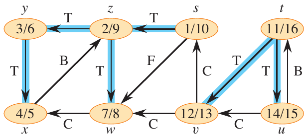
Figure 6: DFS forest from Cormen et al.
The edges are labeled as either
- tree edges: edges in the depth-first forest.
- back edges: edges that point from a vertex to an ancestor in the depth-first forest.
- forward edges: edges that point from a vertex to a descendant in the depth-first forest.
The above graph can be visualized as a DFS forest, as shown below.
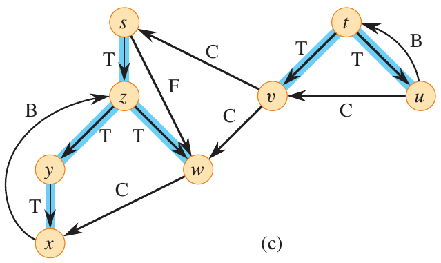
Figure 7: DFS forest from Cormen et al.