Lagrangian Multipliers
Introduction
Let’s take a simple constrained problem (from Nocedal and Wright).
\begin{align*} \min \quad & x_1 + x_2\\ \textrm{s.t.} \quad & x_1^2 + x_2^2 - 2 = 0 \end{align*}
The set of possible solutions to this problem lie on the boundary of the circle defined by the constraint:
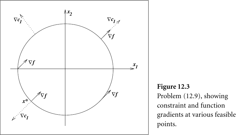
Figure 1: Source: Nocedal and Wright
If we let \(g(\mathbf{x}) = x_1^2 + x_2^2 - 2\), then the gradient vector is \((2x_1, 2x_2)\)
Our original function \(f(\mathbf{x}) = x_1 + x_2\) has a gradient vector of \((1, 1)\).
The figure above visualizes these vectors at different points on the constraint boundary.
Notice that the optimal solution \(\mathbf{x}^* = (-1, -1)\) is at a point where \(\nabla g(\mathbf{x}^*)\) is parallel to \(\nabla f(\mathbf{x}^*)\). However, the gradients of the vectors are not equal. So there must be some scalar \(\lambda\) such that \(\nabla f(\mathbf{x}^*) = \lambda \nabla g(\mathbf{x}^*)\).
This scalar \(\lambda\) is called a Lagrangian multiplier. We use this and introduce the Lagrangian function:
\begin{equation*} \mathcal{L}(\mathbf{x}, \lambda) = f(\mathbf{x}) - \lambda g(\mathbf{x}) \end{equation*}
This yields a form for which we can analytically calculate the stationary points. That is,
\begin{equation*} \nabla_{\mathbf{x}} \mathcal{L}(\mathbf{x}^*, \lambda^*) = 0. \end{equation*}
Lagrangian Duality
In general, the primal optimization problem is formulated as
\begin{align*} \min_{w} \quad & f(w)\\ \textrm{s.t.} \quad & g_i(w) \leq 0, \quad i = 1, \dots, k\\ & h_i(w) = 0, \quad i = 1, \dots, l. \end{align*}
The Lagrangian function is then
\[ L(w, \alpha, \beta) = f(w) + \sum_{i=1}^k\alpha_i g_i(w) + \sum_{i=1}^l \beta_i h_i(w). \]