Linear Filters
Liner filters are a fundamental concept in computer vision. They are used to process images in a variety of ways, such as smoothing, sharpening, and edge detection. They are also used in convolutional neural networks to extract features from images. An essential building block of the computer vision pipeline, understanding linear filters is crucial for anyone working in the field.
Smoothing
When discussing resizing and interpolation, we saw how the choice of scale factor and rotation can produce aliasing in images. Typically, this effect is hidden using some sort of smoothing.
Let’s first look at the case of downsampling an image to 10\% of its original size. If we use nearest neighbor interpolation, the result is very blocky, as seen below.
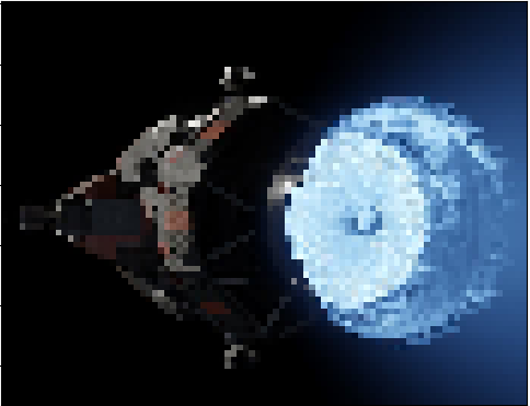
Figure 1: Rocinante cropped and scaled to 10% of the original size. Source: The Expanse
Effectively, an entire block of pixels in the original image is being mapped to the nearest neighbor. We are losing a lot of information from the original image. The figure below shows an overlay of the low resolution grid over a patch of the high resolution image.
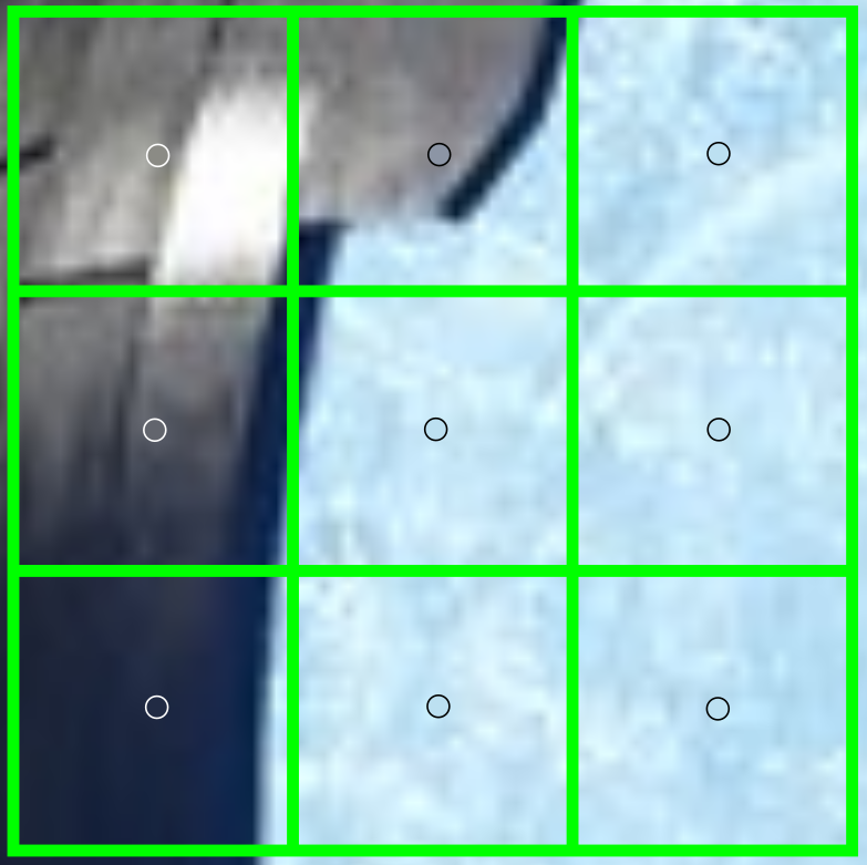
Figure 2: The center dots show the selected pixel value for the downsampled grid.
Computing the Average
Instead of naively selecting one pixel to represent an entire block, we could compute the average pixel value of all pixels within that block. This is a simple as taking an equal contribution from each pixel in the block and dividing by the total number of pixels in the block. An example of such a block is shown below.

Figure 3: A (3 times 3) averaging filter.
By varying the size of this filter, we can effectively change the factor for which we smooth the aliasing.

Figure 4: Original image smoothed with (9 times 9) average filter before downsampling to 10% of its original size.
Convolution
How can we apply the averaging filter to an image effectively? We slide the filter across the image starting at the first pixel in the first row and move row by row until all pixels have been computed.
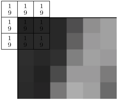
Figure 5: The takes input from all pixels under it and computes the average.
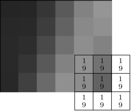
Figure 6: Final portion of image after kernel is applied.
This is performed by the convolution operation. It is defined as
\begin{equation*} g(x, y) = \omega * f(x, y) = \sum_{dx = -a}^a \sum_{dy=-b}^b \omega(dw, dy)f(x + dx, y + dy). \end{equation*}
The range \((-a, a)\) represents the rows of the kernel and \((-b, b)\) the range of the columns of the kernel. The center of the kernel is at \((dx = 0, dy = 0)\).
This operation is one of, if not the most, important operations in computer vision. It is used to apply filters, but we will later see it as one of the guiding operators for feature extraction and deep learning methods.
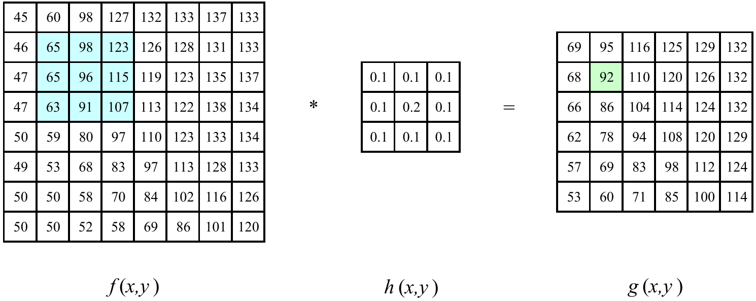
Figure 7: An image (f) convolved with kernel (h). Source: Szeliski
Properties
Commutativity
\(f * g = g * f\)
Associativity
\(f * (g * h) = (f * g) * h\)
Distributivity
\(f * (g + h) = (f * g) + (f * h)\)
Shift Invariant Linear Systems
Convolution is a linear shift-invariant operator. That is, it obeys the following properties.
Superposition: The response of the sum of the input is the sum of the individual responses.
\[ R(f + g) = R(f) + R(g) \]
Scaling: The response to a scaled input is equal to the scaled response of the same input.
\[ R(kf) = kR(f) \]
Shift Invariance: The response to a translated input is equal to the translation of the response to the input.
A system is linear if it satisfies both the superposition and scaling properties. Further, it is a shift-invariant linear system if it is linear and satisfies the shift-invariance property.
Is the average box filter linear? Yes, it is applied with convolution which behaves the same everywhere.
Is thresholding a linear system? No, it can be shown that \(f(n, m) + g(n, m) > T\), but \(f(n, m) < T\) and \(g(n, m) < T\).
Why Is This Important?
In the context of computer vision, this property has very important practical implications. For example, convolutions are used to identify common image features in a Convolutional Neural Network. This property ensures that the feature will be detected regardless of its absolute position in the image. This is critical for tasks like object recognition, where the same feature can appear anywhere in the input.
Gaussian Filters
Blurring an image using a box filter does not simulate realistic blurring as well as Gaussian filters do. The following figure exemplifies the difference between the two.
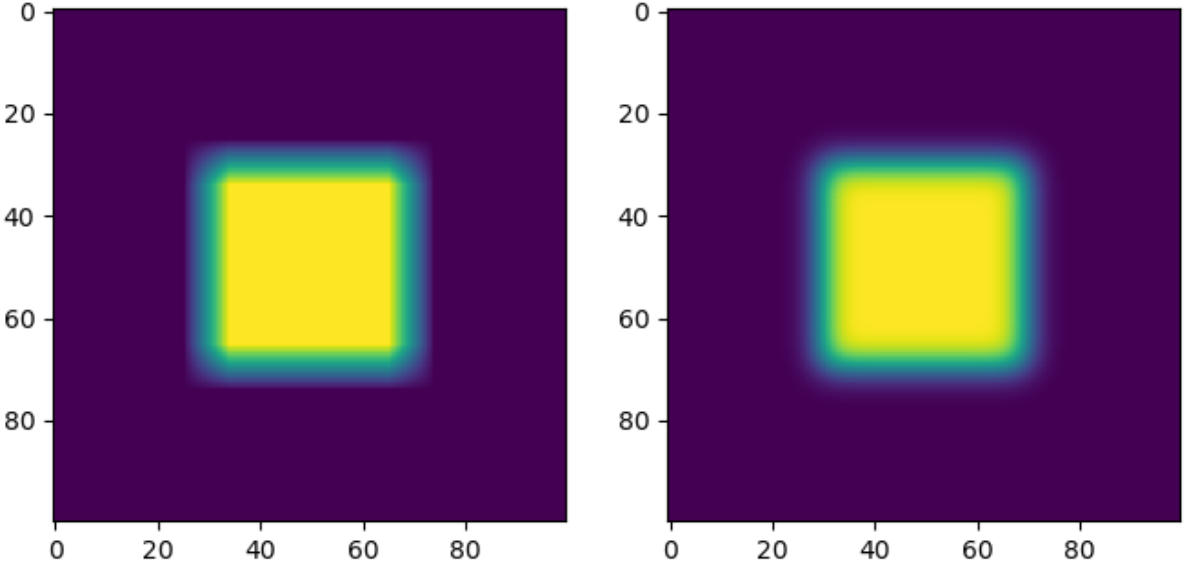
Figure 8: The left image is blurred using a uniform average box filter. The right image is blurred with a Gaussian filter.
The shortcomings of the average box filter can be seen when viewing the artifacting visible at edges, especially at corners.
A Guassian kernel is defined as
\begin{equation*} G(x, y;\sigma) = \frac{1}{2\pi \sigma^2}\exp\Big(-\frac{(x^2 + y^2)}{2 \sigma^2}\Big). \end{equation*}
In effect, it enforces a greater contribution from neighbors near the pixel and a smaller contribution from distant pixels.
Image Derivatives
We can use convolution to approximate the partial derivative (or finite difference) of an image. Recall that
\begin{equation*} \frac{\partial f}{\partial x} = \lim\limits_{\epsilon \rightarrow 0} \frac{f(x + \epsilon, y) - f(x, y)}{\epsilon}. \end{equation*}
We can estimate this as a finite difference
\begin{equation*} \frac{\partial h}{\partial x} \approx h_{i+1, j} - h_{i-1, j}. \end{equation*}
Which can be applied via convolution given a kernal
\begin{equation*} \mathcal{H} = \begin{bmatrix} 0 & 0 & 0\\ -1 & 0 & 1\\ 0 & 0 & 0\\ \end{bmatrix}. \end{equation*}
Applying both the horizontal and vertical derivative kernels to an image to a simple square shows the detection of horizontal and vertical edges.
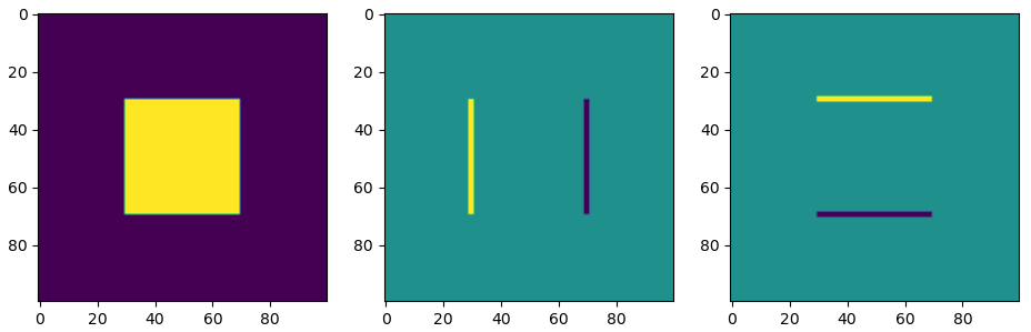
Figure 9: Horizontal (right) and vertical (middle) derivative kernels applied to the original image (left).
The results of applying the derivative kernels are referred to as vertical edge and horizontal edge scores. Consider the middle image in the figure above. The left edge has pixel values of 255; the right edge has -255. In either case, a high absolute score reveals that there is an edge. These scores report the direction of greatest change. The 255 on the left edge indicates the direction is to the right, while the -255 score indicates the direction is to the left. All other instances of the image return a rate of change of 0. Let’s see how these filters perform on a more interesting image.
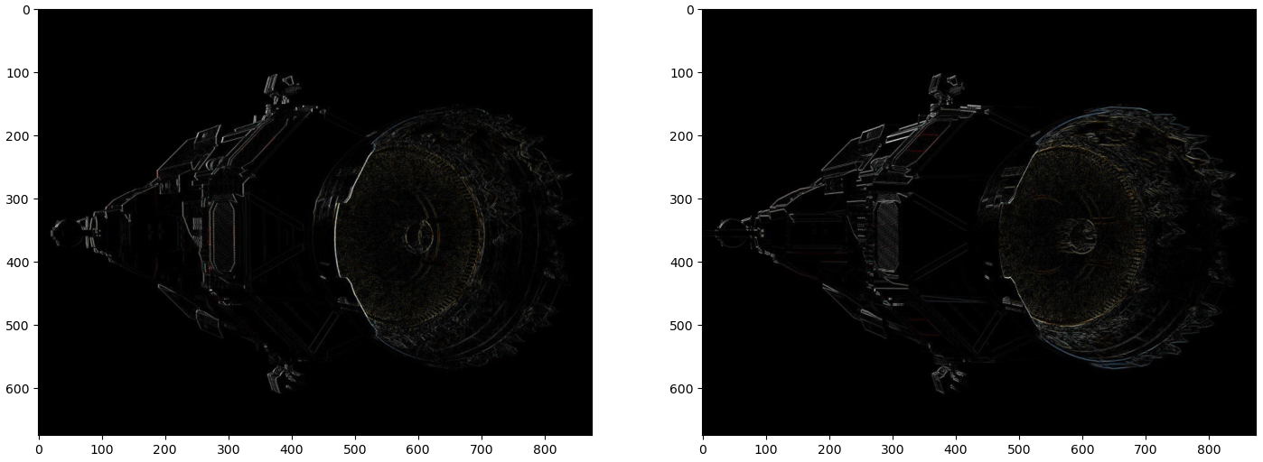
Figure 10: Vertical derivative filter (left) and horizontal derivative filter (right).