Long Short-Term Memory
The recurrent nature of RNNs means that gradients get smaller and smaller as the timesteps increase. This is known as the vanishing gradient problem. One of the first popular solutions to this problem is called Long Short-Term Memory, a recurrent network architecture by Hochreiter and Schmidhuber.
An LSTM is made up of memory blocks as opposed to simple hidden units. Each block is differentiable and contains a memory cell along with 3 gates: the input, output, and forget gates. These components allow the blocks to maintain some history of information over longer range dependencies.
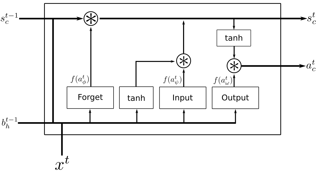
Figure 1: LSTM memory block with a single cell (adapted from Andrew Ng’s diagram).
The original LSTM only had an input and output gate. Forget gates were added in 2000 by Gers et al. to control the amount of context that could be reset, if the task called for it. Peephole connections were proposed by Gers et al. in 2002. These are weights that combine the previous cell state to the gates in order to learn tasks that require precise timing.
By controlling when information can either enter or leave the memory cell, LSTM blocks are able to maintain more historical context than RNNs.
Forward Pass
The equations listed here follow notation and description from Alex Graves’ thesis.
The weight from unit \(i\) to \(j\) is given as \(w_{ij}\). The input to unit \(j\) at time \(t\) is \(a_j^t\) and the result of its activation function is \(b_j^t\). Let \(\psi\), \(\phi\), and \(\omega\) be the input, forget, and output gates. A memory cell is denoted by \(c \in C\), where \(C\) is the set of cells in the network. The activation, or state, of a given cell \(c\) at time \(t\) is \(s_c^t\). The output of each gate passes through an activation function \(f\), while the input and output activation functions of a memory block are given by \(g\) and \(h\).
The forward pass for the input gates is
\[ a_{\psi}^t = \sum_{i=1}^I w_{i\psi}x_i^t + \sum_{h=1}^H w_{h\psi}b_h^{t-1} + \sum_{c=1}^C w_{c\psi}s_c^{t-1}. \]
The output of the forget gates is
\[ a_{\phi}^t = \sum_{i=1}^I w_{i\phi}x_i^t + \sum_{h=1}^H w_{h\phi}b_h^{t-1} + \sum_{c=1}^C w_{c\phi}s_c^{t-1}. \]
The output of the output gates is
\[ a_{\omega}^t = \sum_{i=1}^I w_{i\omega}x_i^t + \sum_{h=1}^H w_{h\omega}b_h^{t-1} + \sum_{c=1}^C w_{c\omega}s_c^{t-1}. \]
Each of the outputs above is passed through an activation function \(f\).
The output of each cell is computed as
\[ a_c^t = \sum_{i=1}^I w_{ic}x_i^t + \sum_{i=1}^H w_{hc}b_h^{t-1} \]
and the internal state is updated via
\[ s_c^t = b_{\phi}^t s_c^{t-1} + b_{\psi}^t g(a_c^t). \]
The state update considers the state at the previous timestep multiplied by the output of the forget gate. That is, it controls how much of the current memory to keep.
The final cell output is given as
\[ b_c^t = b_{\omega}^t h(s_c^t). \]