Markov Decision Processes
Key Terms
- Agent: The learner or decision maker.
- Environment: The world that the agent can interact with.
- State: A representation of the agent and environment.
- Action: The agent can take an action in the environment.
- Reward: Given to the agent based on actions taken.
Goal: Maximize rewards earned over time.
At time \(t\), the agent observes the state of the environment \(S_t \in \mathcal{S}\) and can select an action \(A_t \in \mathcal{A}(s)\), where \(\mathcal{A}(s)\) suggests that the available actions are dependent on the current state. At time \(t + 1\), the agent receives a reward \(R_{t+1} \in \mathcal{R}\).
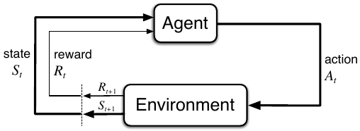
Figure 1: The agent-environment in a Markov decision process (Credit: Sutton & Barto).
To improve its knowledge about an environment or increase its performance on a task, an agent must first be able to interpret or make sense of that environment in some way. Second, there must be a well defined goal. For an agent playing Super Mario, for example, the goal would be to complete each level while maximizing the score. Third, the agent must be able to interact with its environment by taking actions. If the Mario-playing agent could not move Mario around, it would never be able to improve. If the agent makes a decision which leads to Mario’s untimely demise, it would update its knowledge of the world so that it would tend towards a more favorable action. These three requirements: sensations, actions, and goals, are encapsulated by Markov Decision Processes.
A Markov decision process is defined by
- \(\mathcal{S}\) - a set of states,
- \(\mathcal{A}\) - a set of actions,
- \(\mathcal{R}\) - a set of rewards,
- \(P\) - the transition probability function to determine transition between states,
- \(\gamma\) - discount factor for future rewards.
At time \(t\), an agent in state \(S_t\) selects an action \(A_t\). At \(t+1\), it receives a reward \(R_{t+1}\) based on that action.
In a finite MDP, the states, actions, and rewards have a finite number of elements. Random variables \(R_t\) and \(S_t\) have discrete probability distributions dependent on the preceding state and action.
\[ p(s’, r|s, a) = P\{S_t = s’, R_t = r|S_{t-1} = s, A_{t-1} = a\} \]
If we want the state transition probabilities, we can sum over the above distribution:
\[ p(s’|s, a) = P\{S_t = s’|S_{t-1} = s, A_{t-1}=a\} = \sum_{r\in\mathcal{R}}p(s’, r|s, a). \]
The reward function \(r\) gives the expected next reward given some state and action:
\[ r(s, a) = \mathbb{E}[R_{t+1}|S_t=s, A_t=a] = \sum_{r}r \sum_{s’}p(s’, r|s, a). \]
Defining Goals
In reinforcement learning, the goal is encoded in the form of a reward signal. The agent sets out to maximize the total amount of reward it receives over an episode. An episode is defined dependent on the problem context and ends in a terminal state. It could be a round of game, a single play, or the result of moving a robot. Typically, the rewards come as a single scalar value at teach time step. This implies that an agent might take an action that results in a negative reward if it is optimal in the long run.
Formally, the expected return includes a discount factor that allows us to control the trade-off between short-term and long-term rewards:
\[ G_t = \sum_{k=0}^{\infty} \gamma^k R_{t+k+1}, \]
where \(0 \leq \gamma \leq 1\). This can be written in terms of the expected return itself as well:
\[ G_t = R_{t+1} + \gamma G_{t+1}. \]
Policies and Values
Two important concepts that help our agent make decisions are the policy and value functions. A policy, typically denoted by \(\pi\), maps states to actions. Such a function can be deterministic, \(\pi(s) = a\), or stochastic, \(\pi(a|s)\).
The value of a particular state under a policy \(\pi\) is defined as
\[ v_{\pi}(s) = \mathbb{E}_{\pi}[G_t | S_t = s] = \mathbb{E}_{\pi}\Bigg[\sum_{k=0}^{\infty}\gamma^k R_{t+k+1}\Bigg|S_t=s\Bigg]. \]
We also must define the value of taking an action \(a\) in state \(s\) following policy \(\pi\):
\[ q_{\pi}(s, a) = \mathbb{E}_{\pi}[G_t|S_t=s, A_t=a] = \mathbb{E}_{\pi}\Bigg[\sum_{k=0}^{\infty}\gamma^k R_{t+k+1}\Bigg|S_t=s, A_t=a\Bigg]. \]
This function defines the expected return of following a particular policy and starting in state \(s\). Both the state-value and action-value functions can be updated as a result of the agent’s experience. How it is updated is method-dependent. Certain methods will also dictate how the policy itself can be updated.
Bellman Equations
The recursive relationship between the value of a state and its future states can be represented using Bellman equations. In RL, we are interested in the equations for both the state-value and action-value. Given the diagram of an MDP, we can see that they are related to each other. To make the following equations easier to understand, it is important to remember the flow of a Markov decision process:
- take an action,
- arrive at a state and sense the reward,
- consult the policy for the next action.
With that in mind, let’s look at the state-value function first. This function considers the expected value of starting in a state \(s\) and following policy \(\pi\). In other words, we must consider all possible actions and their future rewards.
\begin{align*} v_{\pi}(s) &= \mathbb{E}_{\pi}[G_t | S_t = s]\\ &= \mathbb{E}_{\pi}[R_{t+1} + \gamma G_{t+1} | S_t = s]\\ &= \sum_{a} \pi(a|s) \sum_{s’}\sum_{r}p(s’, r|s, a)\Big[r + \gamma \mathbb{E}_{\pi}[R_{t+1} + \gamma G_{t+1} | S_t = s]\Big]\\ &= \sum_{a} \pi(a|s) \sum_{s’, r}p(s’, r|s, a)\Big[r + \gamma v_{\pi}(s’)\Big]\\ &= \sum_{a} \pi(a | s)\big[r(s, a) + \gamma \sum_{s’}p(s’|s, a)v_{\pi}(s’)\big]\\ \end{align*}
The first sum over actions considers all possible actions. This is followed by a transition to possible states \(s’\) conditioned on taking each action multiplied by the expected value of being at the new state.
The action-value function follows a similar derivation:
\begin{align*} q_{\pi}(s, a) &= \mathbb{E}_{\pi}[G_t|S_t = s, A_t = a]\\ &= \mathbb{E}_{\pi}[R_{t+1} + \gamma G_{t+1} | S_t = s, A_t = a]\\ &= r(s, a) + \sum_{s’}p(s’|s, a) v_{\pi}(s’) \end{align*}
There is a very similar looking set of terms in the state-value function above, and we should expect that! If we want to evaluate the current state, we need to look ahead at the possible actions and their resulting rewards. Similarly, evaluating the current action requires us to look head at the value of future states.
Let’s expand \(q_{\pi}(s,a)\) once more so that it is written in terms of itself.
\begin{align*} q_{\pi}(s, a) &= r(s, a) + \gamma \sum_{s’}p(s’|s, a) v_{\pi}(s’)\\ &= r(s, a) + \gamma \sum_{s’}p(s’|s, a) \sum_{a’} \pi(s’, a’) \big[r(s’, a’) + \gamma \sum_{s’’} p(s’’|s’, a’)v_{\pi}(s’’)]\\ &= r(s, a) + \gamma \sum_{s’}p(s’|s, a) \sum_{a’} \pi(s’, a’) q_{\pi}(s’, a’) \end{align*}
Optimality
To solve a reinforcement learning problem, we are interested in finding the policy \(\pi_{*}\) whose expected return is greater than all other possible policies over all states. An optimal policy will use an *optimal state-value function and optimal action-value function:
\begin{align*} v_{*}(s) &= \max_{\pi}v_{\pi}(s)\\ q_{*}(s, a) &= \max_{\pi}q_{\pi}(s, a). \end{align*}
The optimal state-value function would select the best possible action instead of summing over all possibley actions starting in state \(s\):
\begin{align*} v_{*}(s) &= \max_{a} q_{\pi_*}(s, a)\\ &= \max_{a}\big[r(s, a) + \gamma \sum_{s’} p(s’|s, a) v_{*}(s’)\big] \end{align*}
Similarly, the optimal action-value function selects the best possible action from the next state \(s’\):
\[ q_{*}(s) = r(s, a) + \gamma \sum_{s’} p(s’|s, a) \max_{a} q_{*}(s’, a’). \]
Optimizing the Policy
For smaller problems with reasonably small state and action spaces, we can use Dynamic Programming to compute the optimal policy. These methods quickly become intractable as the complexity of our problem increases. As is common in machine learning, we would resort to approximation methods for complex spaces.
“In fact, all of these methods can be viewed as attempts to achieve much the same effect as DP, only with less computation and without assuming a perfect model of the environment.”
– Richard S. Sutton and Andrew G. Barto, Reinforcement Learning: An Introduction
Imagine if you had a set policy that dictated the actions you would take from work to home. In this example, assume the policy is not an optimal policy. One day, you decide to take a left at a particular intersection rather than going forward. After that, you follow your policy as described. If this decision ultimately resulted in you arriving home sooner, you would probably update your policy to always take that left. This intuition describes a result of the policy improvement theorem.
Let \(\pi\) and \(\pi’\) be two deterministic policies where
\[ q_{\pi}(s, \pi’(s)) \geq v_{\pi}(s),\quad \forall s. \]
We can reasonably conclude that, in this case, \(\pi’\) must be at least as good as \(\pi\).