Maximum Flow
The slides accompanying these notes can be found here.
A flow network is a directed graph in which the edges begin at a node that produces the flow and the adjacent nodes are the ones that receive it. Flow in this context could take on many meanings, such as the amount of water that can flow through a pipe, the amount of data that can be sent through a network, or the amount of traffic that can be sent through a road network. The goal of a flow network is to maximize the flow from the source to the sink.
The problem may have intermediate constraints. For example, a network graph may have a node with limited bandwidth, so the flow through that node must be less than or equal to the bandwidth. These notes review the formal definition of the problem followed by a solution using the Ford-Fulkerson algorithm as well as one related to bipartite matching.
Objective Questions
- What is the maximum flow problem?
- How can we solve it?
Maximum Flow
A flow network \(G = (V, E)\) is a directed graph in which each edge \((u, v) \in E\) has a nonnegative capacity \(c(u, v) \geq 0\). The graph does not contain reverse edges between two vertices. If an edge does not exist in the set, then its capacity is 0. Each graph has a source and a sink, which will be the main edges of note when analyzing the graph. The goal is to maximize the flow going from the source to the sink. This implies that the source has no incoming edges.
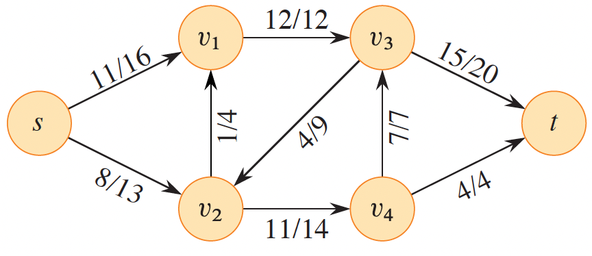
Figure 1: A flow network. Each edge depicts (f(u,v)/c(u,v)), the flow and capacity (Cormen et al. 2022).
A flow in a graph \(G\) is a function \(f : V \times V \rightarrow \mathbb{R}\) that satisfies two properties:
- Capacity constraint: For all \(u, v \in V\), \[ 0 \leq f(u,v) \leq c(u,v). \]
- Flow conservation: For all \(u \in V - \{s, t\}\), \[ \sum_{v \in V} f(v, u) = \sum_{v \in V} f(u, v). \]
There are usually many different possibly paths of flow in a flow network. The maximum flow problem asks: what is the path that yields the maximum flow?
Antiparallel Edges
The restriction that no two nodes may have more than one edge seems to be unrealistic. For example, modeling the flow of a network graph with this restriction means that network traffic can only move in one direction between two datacenters. If there were two edges between adjacent nodes \(v_1\) and \(v_2\) such that \((v_1, v_2) \in E\) and \((v_1, v_2) \in E\), we would call these edges antiparallel. In such cases, the graph is modified with a new node \(v’\) such that \((v_1, v’) \in E\) and \((v’, v_2) \in E\). An example is shown below.
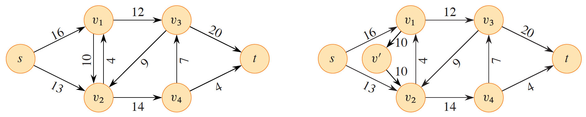
Figure 2: Addressing antiparallel edges in a flow network (Cormen et al. 2022).
Multiple Sources and Sinks
Another restriction that is unrealistic in many real-world scenarios is that maximum flow graphs can only have a single source and sink. It is easy to imagine a scenario where multiple sources and sinks within a network. Again, the graph can be modified to accommodate this scenario by defining a supersource and supersink whose outgoing and incoming flows are infinite.
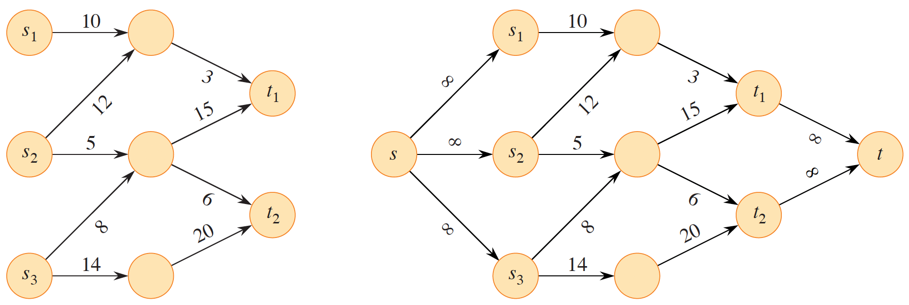
Figure 3: Assing a supersource and supersink to a graph with multiple sources and sinks (Cormen et al. 2022).
A polynomial time solution
Ford-Fulkerson relies on three foundational concepts:
- Residual networks
- Augmenting paths
- Cuts
The solution presented by Ford and Fulkerson is not a single algorithm but rather a set of general instructions.
- Initialize \(f(u, v) = 0\) for all \(u,v \in V\), giving an initial flow of 0.
- Increase the flow by finding an augmenting path in a residual network.
- The edges of the augmented path indicate where to increase the flow.
This is repeated until the residual network has no more augmenting paths.
Residual Networks
Consider a pair of vertices \(u, v \in V\), the residual capacity \(c_f(u, v)\) is amount of additional flow that can be pushed from \(u\) to \(v\).
\[ c_f(u, v)= \begin{cases} c(u,v) - f(u, v)\quad \text{if } (u,v) \in E,\\ f(v, u)\quad \text{if } (v, u) \in E,\\ 0\quad \text{otherwise (i.e., } (u, v), (v, u) \notin E). \end{cases} \]
The residual network is \(G_f = (V, E_f)\), where
\[ E_f= \{(u, v) \in V \times V : c_f(u, v) > 0\}. \]
The edges of \(G_f\) represent those edges in \(G\) with the capacity to change the flow. There is also no requirement for all edges in \(G\) to be present in \(G_f\). As the algorithm works out the solution, we are only considered with edges that permit more flow.
An edge \((u, v) \in E\) means that the reverse edge \((v, u) \notin E\). However, the residual network can have edges that are not in \(G\). These are used to represent paths in which flow is sent in the reverse direction. This can happen if reducing flow from one edge results in a net increase across some other.
In \(G_f\), the reverse edges \((v, u)\) represent the flow on \((u, v) \in G\) that could be sent back.
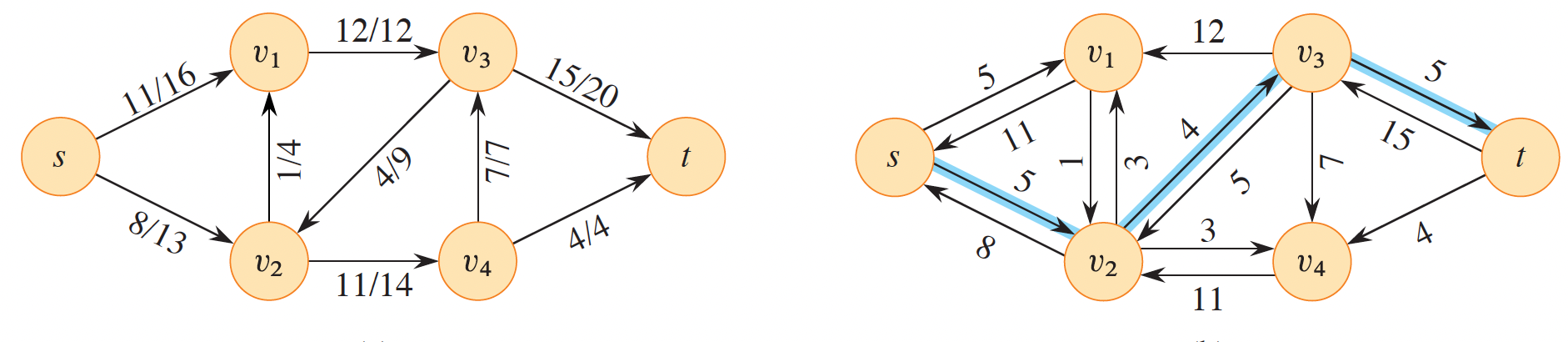
Figure 4: A flow network and its residual network (Cormen et al. 2022).
Augmentation Function
Given flows \(f\) in \(G\) and \(f’\) in \(G_f\), define the augmentation of \(f\) by \(f’\), as a function \(V \times V \rightarrow \mathbb{R}\):
\[ (f \uparrow f’)(u, v) = \begin{cases} f(u, v) + f’(u, v) - f’(u, v)\quad \text{if } (u, v) \in E,\\ 0 \quad \text{otherwise} \end{cases} \]
for all \((u, v) \in V\).
This augmentation function represents an increase of flow on \((u, v)\) by \(f’(u, v)\) with a decrease by \(f’(v, u)\) since pushing flow on the reverse edge in \(G_f\) represents a decrease in \(G\). This is known as cancellation.
Lemma
Given a flow network \(G\), a flow \(f\) in \(G\), and the residual network \(G_f\), let \(f’\) be a flow in \(G_f\). Then \((f \uparrow f’)\) is a flow in \(G\) with value \(|f \uparrow f’| = |f| + |f’|\).
This lemma defines the idea of net flow. If there are 10 units of flow in one direction and 4 in the other, the edge effectively has 6 units of flow.
Augmenting Paths
An augmenting path is a simple path from the source to the sink in the residual network.
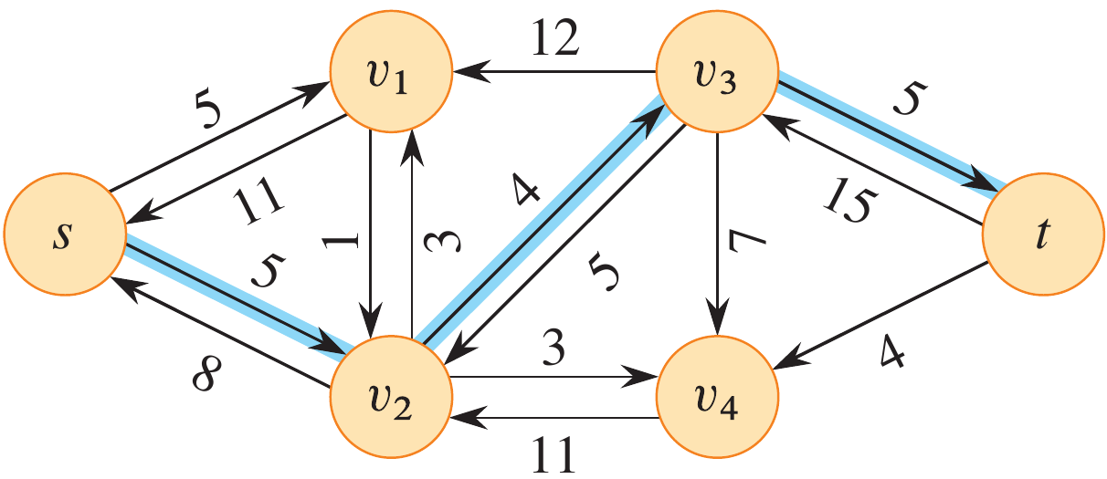
Figure 5: An augmenting path in a flow network (Cormen et al. 2022).
The purpose of an augmenting path is to increase the flow from the source to the sink. The flow is increased by the minimum capacity of the edges in the path.
Lemma 24.2
Let \(G = (V, E)\) be a flow network, let \(f\) be a flow in \(G\), and let \(p\) be an augmenting path in \(G_f\). Define \(f_p : V \times V \rightarrow \mathbb{R}\) by
\[ f_p(u, v) = \begin{cases} c_f(p) & \text{if } (u, v) \text{ is in } p,\\ 0 & \text{otherwise}. \end{cases} \]
Then \(f_p\) is a flow in \(G_f\) with value \(|f_p| > 0\).
The maximum amount that an augmenting path can be increased is the minimum capacity of the edges in the path. This is known as the residual capacity of the path.
\[ c_f(p) = \min \{c_f(u, v) : (u, v) \text{ is in } p\}. \]
Put simply, if there is a path in the residual network, the flow can be increased by the minimum capacity of the edges in the path. If there is no path, the flow is at its maximum.
Cuts
A cut \((S, T)\) of a flow network \(G = (V, E)\) is a partition of \(V\) into two sets \(S\) and \(T = V - S\) such that \(s \in S\) and \(t \in T\). The capacity of the cut is the sum of the capacities of the edges from \(S\) to \(T\). Any cut is a valid cut as long as the source is in \(S\) and the sink is in \(T\).
If \(f\) is a flow in \(G\) and \((S, T)\) is a cut of \(G\), then the net flow across the cut is
\[ f(S, T) = \sum_{u \in S} \sum_{v \in T} f(u, v) - \sum_{u \in S} \sum_{v \in T} f(v, u). \]
The capacity of the cut is
\[ c(S, T) = \sum_{u \in S} \sum_{v \in T} c(u, v). \]
A minimum cut is a cut whose capacity is the smallest among all cuts.
Lemma
For any flow \(f\) and any cut \((S, T)\) of \(G\), we have that $|f| = f(S, T).$
This lemma states that the flow across a cut is equal to the value of the flow.
Proof
\begin{align*} f(S, T) &= f(S, V) - f(S, S)\\ &= f(S, V)\\ &= f(s, V) + f(S - s, V)\\ &= f(s, V) = |f|. \end{align*}
Key concept: We can determine the flow by making cuts in the graph. The minimum cut leads to the maximum flow.
Corollary
The value of any flow \(f\) in a flow network \(G\) is bounded from above by the capacity of any cut of \(G\).
Max-flow Min-cut Theorem
The following statements are logically equivalent.
- The flow \(f\) is a maximum flow in \(G\).
- The residual network \(G_f\) contains no augmenting paths.
- The value of the flow \(f\) is equal to the capacity of the cut \((S, T)\) for some cut of \(G\).
Ford-Fulkerson Algorithm
The Ford-Fulkerson algorithm is a general method for solving the maximum flow problem. The algorithm is not a single algorithm but rather a set of instructions that can be implemented in different ways. The algorithm is as follows:
def ford_fulkerson(G, s, t):
    f = {u: {v: 0 for v in G} for u in G}
    while True:
        # Find an augmenting path
        path = bfs(G, s, t, f)
        if not path:
            break
        cf = min(G[u][v] - f[u][v] for u, v in path)
        for u, v in path:
            f[u][v] += cf
            f[v][u] -= cf
    return f
Example
Run the Ford-Fulkerson algorithm on the following graph.
Analysis
The running time of Ford-Fulkerson hinges on how the augmenting path is found. If implemented with a breadth-first search, the algorithm runs in \(O(VE^2)\) time.
Edmonds-Karp Algorithm
The Edmonds-Karp algorithm is a specific implementation of Ford-Fulkerson that uses breadth-first search to find the augmenting path. The algorithm presented above is actually the Edmonds-Karp algorithm.