Minimum Spanning Trees
The slides accompanying these lectures notes can be found here.
Minimum spanning trees are undirected graphs that connect all of the vertices such that there are no redundant edges and the total weight is minimized. They are useful for finding the shortest path between two points in a graph. Useful application of MSTs include
- network design: it is useful to know the least expensive path with respect to either latency or resource cost for telecommunications networks, transportation networks, or electrical grids.
- approximation algorithms: MSTs can be used to approximate the solution to the traveling salesman problem.
- clustering: MSTs can be used to cluster data points in a graph.
- image segmentation: MSTs can be used to segment images into smaller regions.
Definition
Let \(G\) be a connected, undirected graph with edges \(E\), vertices \(V\), and edge weights \(w\). A minimum spanning tree is a subset \(T \subseteq E\) that connects all of the vertices such that the total weight is minimized. The original graph \(G\) is shown below.
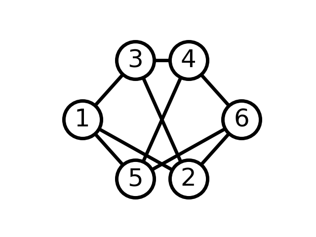
Figure 1: An undirected graph with redundant edges.
The minimum spanning tree of the above graph is show below. All of the redundant edges have been removed, but there is still a path between each pair of nodes.
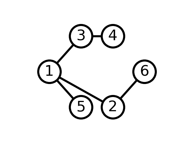
Figure 2: The minimum spanning tree of (G).
As described in Introduction to Algorithms there are two greedy algorithms for finding the minimum spanning tree of a graph (Cormen et al. 2022). These notes will review both of these, but first let’s look at a general algorithm for finding the minimum spanning tree of a graph.
Properties
A minimum spanning tree must satisfy the following properties.
- It has \(|V| - 1\) edges.
- It has no cycles.
- It might not be unique.
Finding the Minimum Spanning Tree
The general algorithm for finding the minimum spanning tree of a graph grows a set of edges \(T\) from an empty set. At each step, the algorithm adds the edge with the smallest weight that does not create a cycle. The algorithm terminates when \(T\) is a complete tree.
T = {}
while T is not a spaning tree
    find the edge e with the smallest weight that does not create a cycle
    T = T union {e}
Each edge \(e\) that is added must result in a tree that is a subset of the minimum spanning tree. The challenge of this algorithm is actually finding such an edge. How would we know such an edge if we saw it? We first need to define a few properties which will shine light on this.
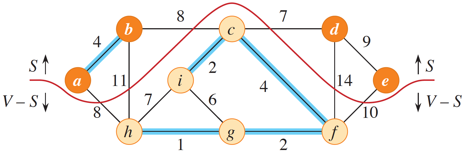
Figure 3: A cut of a graph (Cormen et al. 2022).
A cut of a graph \(G\) is a partition of the vertices \(V\) into two disjoint sets \(S\) and \(V - S\). An edge \(e\) crosses the cut if one of its endpoints is in \(S\) and the other is in \(V - S\). If no edge in a given set \(E\) crosses the cut, then that cut respects \(E\). An edge that is the minimum weight edge that crosses a cut is called a light edge. With these definitions, we can now formally define how to find a safe edge, which is an edge that can be added to the current set of edges \(T\) without creating a cycle.
Theorem 21.1 (Cormen et al. 2022)
Let \(G = (V, E)\) be a connected, undirected graph with a real-valued weight function \(w\) defined on \(E\). Let \(A\) be a subset of \(E\) that is included in some minimum spanning tree for \(G\), let \((S, V - S)\) be any cut of \(G\) that respects \(A\), and let \(e\) be a light edge crossing \((S, V - S)\). Then, edge \(e\) is safe for \(A\).
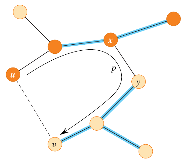
Figure 4: Visual proof of Theorem 21.1 (Cormen et al. 2022).
Proof
The two sets in the figure above represent vertices in \(S\) (orange) and vertices in \(V - S\) (tan). \(T\) is the original MST depicted in the figure. The dotted line is the new edge \((u, v)\) to consider. \(A\) is a subset of edges in \(T\) represented by the blue lines. If the safe edge \((u, v)\) is already in the original MST \(T\), then we are done.
The vertices \(u\) and \(v\) lie on opposite sides of the cut. The edge \((u, v)\) would introduce a cycle since there is already a path from \(u\) to \(v\) in \(T\) that crosses the cut via \((x, y)\). Since both \((u, v)\) and \((x, y)\) are light edges that cross the cut, then it must be that \(w(u, v) \leq w(x, y)\).
Let \(T’\) be the minimum spanning tree with \((x, y)\) replaced by \((u, v)\). That is \(T’ = T - \{(x, y)\} \cup \{(u, v)\}\). Since \(T\) is a minimum spanning tree, then \(w(T) \leq w(T’)\). Since \(w(T) = w(T’)\), then \(T’\) is also a minimum spanning tree. Therefore, \((u, v)\) is safe for \(A\).
Corollary 21.2 (Cormen et al. 2022)
We can also view this in terms of connected components, which are subsets of vertices that are connected by a path. If \(C\) and \(C’\) are two connected components in \(T\) and \((u, v)\) is a light edge connecting \(C\) and \(C’\), then \((u, v)\) is safe for \(T\).
The figure below shows a graph with two individual components. If the edge \((u, v)\) is a light edge, then it is safe to add it to the set of edges \(T\).
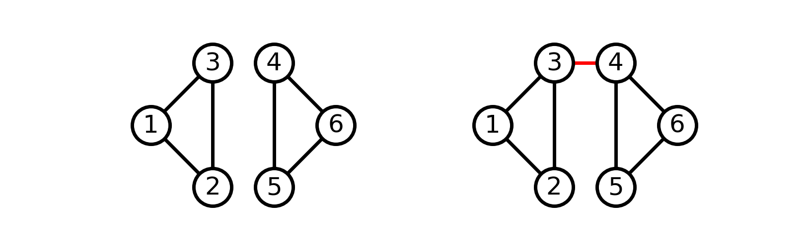
Figure 5: Two connected components from a graph (left). Adding a safe edge (right).
Kruskal’s Algorithm
The first solution to the minimum spanning tree that we will study is called Kruskal’s algorithm. This algorithm grows a forest of trees from an empty set. At each step, the algorithm adds the lightest edge that does not create a cycle. The algorithm terminates when the forest is a single tree. This can be viewed as an agglomerative clustering algorithm. The algorithm starts with each vertex in its own cluster. At each step, the algorithm merges the two clusters that are closest together. The algorithm terminates when there is only one cluster.
The algorithm is given below (Cormen et al. 2022).
Kruskal’s Algorithm
A = {}
for each vertex v in G.V
    MAKE-SET(v)
sort the edges of G.E into nondecreasing order by weight w
for each edge (u, v) in G.E, taken in nondecreasing order by weight
    if FIND-SET(u) != FIND-SET(v)
        A = A union {(u, v)}
        UNION(u, v)
return A
A step-by-step example of an implementation in Python is available here.
Analysis
The running time is dependent on how the disjoint-set of vertices is implemented. In the best known case, a disjoint-set-forest implementation should be used (Cormen et al. 2022). Creating a list of edges takes \(O(E)\) time. Sorting the edges takes \(O(E \log E)\) time. The for loop iterates over each edge, which is \(O(E)\). All disjoin-set operations take \(O((V + E)\alpha(V))\) time. Since the graph is connected, \(E \geq V - 1\), so the total running time is \(O(E \log E + E + E \alpha(V)) = O(E \log E + E \alpha(V)) = O(E \log V)\).
Prim’s Algorithm
The second solution starts at an arbitrary vertex in a set \(A\) and adds a new vertex to \(A\) in a greedy fashion. To efficiently select a new edge to add, Prim’s algorithm uses a priority queue to keep track of the lightest edge that crosses the cut. The algorithm terminates when \(A\) is a complete tree. The full algorithm is given below. We will step through it in more detail after.
Prim’s Algorithm
A = {}
for each vertex v in G.V
    key[v] = infinity
    pi[v] = NIL
key[r] = 0
Q = G.V
while Q is not empty
    u = EXTRACT-MIN(Q)
    A = A union {u}
    for each vertex v in G.Adj[u]
        if v in Q and w(u, v) < key[v]
            pi[v] = u
            key[v] = w(u, v)
You might look at this and wonder how the MST is represented. Prim’s algorithm implicitly maintains the set \(A = \{(v, v.\pi) : v \in V - \{r\} - Q\}\). When the while loop terminates, \(A = \{(v, v.\pi) : v \in V - \{r\}\}\), since the queue is empty. The critical part of this is to understand how the algorith changes the key values.
A step-by-step example of an implementation in Python is available here.
Analysis
Prim’s algorithm uses a priority queue to keep track of the lightest edge that crosses the cut. If the priority queue is implemented as a min-heap, which has a worst-case running time of \(O(\log V)\) for both EXTRACT-MIN and DECREASE-KEY. The algorithm calls EXTRACT-MIN once for each vertex, which is \(O(V \log V)\). The algorithm calls DECREASE-KEY once for each edge, which is \(O(E \log V)\). The total running time is \(O(V \log V + E \log V) = O(E \log V)\).