Multidimensional Grids and Data
Lectures slides for these notes can be found here.
Summary
The CUDA Programming model allows us to organize our data in a multidimensional grid. The purpose of this is primarily for our own convenience, but it also allows us to take advantage of the GPU’s memory hierarchy. In Lab 0, we only required a single dimension for our grid as well as each block since the input was a vector. When performing computations on multidimensional data like matrices, we can match the dimensions of our launch configuration to the dimensions of our data.
Multidimensional Grid Organization
All threads share a block index, blockIdx, and a thread index, threadIdx. These indices are three-dimensional vectors of type dim3. The dim3 type is defined as follows:
struct dim3 {
    unsigned int x, y, z;
};
Each grid is a 3D array of blocks, and every block a 3D array of threads. Consider the kernel execution for vecAdd from Lab 0:
dim3 blocksPerGrid(32, 1, 1);
dim3 threadsPerBlock(128, 1, 1);
vecAdd<<<blocksPerGrid, threadsPerBlock>>>(a_d, b_d, c_d, n);
This will execute with \(32 \times 128 = 4096\) threads.
If our input is a matrix, we should organize our launch dimensions to match its 2D structure. We seemingly have two options: either the grid size or the block size. Consider the figure below, there are 4 blocks in the grid, each with 16 threads organized as a \(4 \times 2 \times 2\) volume.
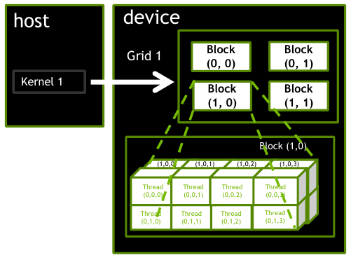
Figure 1: A 2D grid of blocks, each with 16 threads arranged in a 3D configuration (source: NVIDIA DLI).
Under such a configuration, we would make use of gridDim.x, gridDim.y, and gridDim.z to access the dimensions of the grid. The dimensions of the block would be accessed with blockDim.x, blockDim.y, and blockDim.z. The thread indices would be accessed with threadIdx.x, threadIdx.y, and threadIdx.z. Would this be the best way to organize our launch configuration? Not exactly. We have no use for the 3D structure if we are only working with matrices.
Consider an \(n \times m\) matrix. If the matrix is small enough, we could launch a single block with a 2D arrangement of threads to perform the necessary computation. For larger matrices, we would optimally split the work into multiple blocks. This would allow us to perform more work in parallel. Let \(n=62\) and \(m=76\). If we chose a \(16 \times 16\) block size, we would need \(4 \times 5 = 20\) blocks to cover the entire matrix, as shown in the figure below.
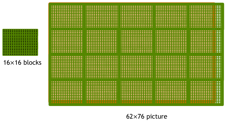
Figure 2: A 2D grid of blocks, each with 16 threads arranged in 2D (source: NVIDIA DLI).
Notes on Compute Capability
It is more important to dynamically adjust the grid size so that your program can adapt to varying input sizes. As of CC 9.0, the maximum number of threads a block can have is 1024, this means that a \(32 \times 32\) block is the largest we can do for matrix data.
If the input matrix is smaller than \(32 \times 32\), then only a single block is needed. The additional threads allocated to that block will be inactive for indices outside the range of our input.
If the input matrix is larger than \(32 \times 32\), additional blocks should be added to the grid to accommodate the increased size. It is safe to keep the block size fixed, but the grid size must be dynamic.
Optimal Launch Parameters
Is it better to have fewer blocks that maximize the amount of threads per block? Or is it better to have more blocks with fewer threads per block? The current maximum number of threads per block is 1024. In practice, a maximum block dimension size of 128 or 256 is ideal. This has more to do with the specific problem and the amount of shared memory required. You will explore this question in Lab 1.
Example: Color to Grayscale
Given the layout just described, we will write a kernel that converts a color image to grayscale. This is an embarrassingly parallel problem since each pixel can be converted independently of the others. We will use the following formula to convert each pixel:
gray = 0.299f * red + 0.587f * green + 0.114f * blue
A CPU implementation would require a for loop over the exact number of pixels. The CUDA kernel for this is straightforward since it only depends on the current pixel. The only real challenge is to compute the correct indices for each thread.
__global__
void colorToGrayscale(unsigned char *rgbImage,
                      unsigned char *grayImage,
                      int numRows, int numCols)
{
    int x = blockIdx.x * blockDim.x + threadIdx.x;
    int y = blockIdx.y * blockDim.y + threadIdx.y;
    if (x >= numCols || y >= numRows) return;

    int index = y * numCols + x;
    int rgbOffset = index * 3;
    unsigned char r = rgbImage[rgbOffset];
    unsigned char g = rgbImage[rgbOffset + 1];
    unsigned char b = rgbImage[rgbOffset + 2];
    float channelSum = 0.299f * r + 0.587f * g + 0.114f * b;
    grayImage[index] = channelSum;
}
In this example, we assume an RGB image where each pixel is represented by three unsigned characters. It is standard convention in C to pass a pointer to the first element of the array. This implies that we cannot use the [] operator to access the elements in a multidimensional way. Instead, we must compute the index ourselves. If you are not currently familiar with flat indexing, you certainly will be by the end of this course.
In C, multi-dimensional arrays are stored in row-major order. To compute the index of row j and column i in a 2D array, we need to skip over j rows and i columns. The total number of columns is the width of the array. The total number of rows is the height of the array. The index is computed as follows:
int index = j * width + i;
This is represented in the following figure.
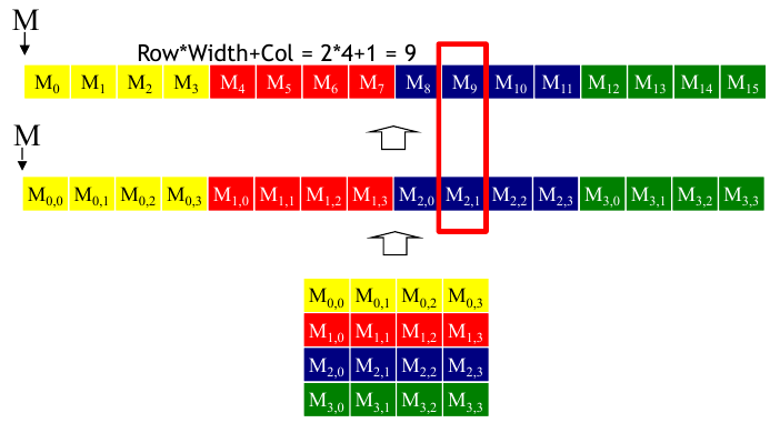
Figure 3: A 2D array stored in row-major order (source: NVIDIA DLI).
Since the image is now represented as a flat 1D array, we can use the index computed above to access the correct pixel. The image is typically stored in the same row-major format, although this is not always the case. You should always check the documentation for the image format you are using.
Launch Configuration
As stated above, we are going to launch 20 blocks in a \(4 \times 5\) grid. Each block will have 256 threads arranged in a \(16 \times 16\) 2D configuration. This totals to \(20 \times 256 = 5120\) threads. The example figure above shows this configuration overlaid on a \(76 \times 62\) image. That means we have 4712 pixels that need to be converted. The remaining 408 threads will be idle.
You might be wondering if all 5120 threads launch at the same time. What if the number of pixels exceeded the number of threads available on the GPU? The short answer is that the GPU will launch as many threads as possible, but the long answer is slightly more complicated and will be discussed in a later lesson.
In any case, our kernel can be launched using the following code:
dim3 blockSize(16, 16, 1);
dim3 gridSize(4, 5, 1);
colorToGrayscale<<<gridSize, blockSize>>>(rgbImage, grayImage, numRows, numCols);
No longer embarrassing: overlapping data
At this point, you should have a basic understanding of how to solve problems that are embarrassingly parallel. Now comes the next step in shaping your parallel thinking skills. What if the thread relies on multiple data points that may be used by other threads? This is further complicated with problems that require some computation to complete before a thread can begin its work. Let’s take a step into deeper waters by looking at image blurring. This is a common technique used in image processing to reduce noise and detail. The basic idea is to replace each pixel with a weighted average of its neighboring pixels. The size of the neighborhood is called the kernel size. The kernel size is typically an odd number so that the pixel of interest is in the center of the neighborhood.
The core operation behind blurring is called a convolution. We will explore this operation in depth as it serves as a more advanced pattern for parallelism. For now, we will focus on the basic idea. Given a kernel size of \(5 \times 5\) centered on a pixel, we will compute the weighted average of the 25 pixels in the neighborhood. To keep it simple, the weights will be uniform.
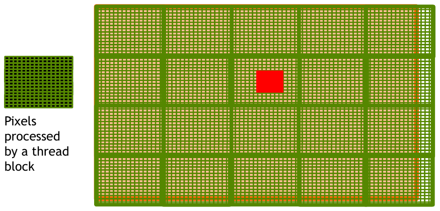
Figure 4: A blurring kernel (red) centered on a pixel (source: NVIDIA DLI).
Given a pixel location \((x, y)\), we can compute the index of the pixel in the neighborhood as follows:
int index = (y + ky) * numCols + (x + kx);
Where \(ky\) and \(kx\) are the row and column indices of the kernel. The kernel is centered on the pixel of interest, so \(ky\) and \(kx\) range from \(-2\) to \(2\). The total number of pixels in the neighborhood is \(5 \times 5 = 25\). The weighted average is computed as follows:
float sum = 0.0f;
int numPixels = 0;
for (int ky = -2; ky <= 2; ky++) {
    for (int kx = -2; kx <= 2; kx++) {
        if (x + kx < 0 || x + kx >= numCols) continue;
        if (y + ky < 0 || y + ky >= numRows) continue;
        int index = (y + ky) * numCols + (x + kx);
        sum += image[index];
        numPixels++;
    }
}
image[y * numRows + x] = sum / numPixels;
Some extra care will be needed to account for pixels outside the boundaries. There are several strategies to handle out-of-bounds pixels. The simplest is to ignore them. We will explore other strategies when discussing convolutions. In Lab 1, you will implement a blur kernel that can support a varying kernel size.
Matrix Multiplication
Matrix multiplication is one of the most important operations in linear algebra. Many high performance computing applications rely on it. It is one of the most widely called operations in deep learning, for example. Parallelizing this and other linear algebra operations has resulted in an explosion of research and applications ranging from computer vision to computational fluid dynamics. Exploring the parallelism of matrix multiplication will give us a deeper understanding of the CUDA programming model. It will also serve as a jumping off point for more advanced topics like shared memory and convolutional neural networks.
Definition
Let \(A = \mathbb{R}^{m \times n}\) and \(B = \mathbb{R}^{n \times p}\) be two matrices. The product \(C = AB\) is defined as follows:
\[ C_{ij} = \sum_{k=1}^n A_{ik} B_{kj}\quad \text{for } i = 1, \ldots, m \text{ and } j = 1, \ldots, p \]
This operation is only defined on compatible matrices. That is, the number of columns in \(A\) must equal the number of rows in \(B\). The resulting matrix \(C\) will have \(m\) rows and \(p\) columns.
CPU Implementation
The CPU implementation of matrix multiplication is straightforward. There is a double for loop to iterate through each element in the output matrix. The inner loop computes the dot product of the $i$th row of \(A\) and the $j$th column of \(B\). The dot product is computed by summing the element-wise product of the two vectors.
void matrixMultiplyCPU(float *A, float *B, float *C, int m, int n, int p) {
    for (int i = 0; i < m; i++) {
        for (int j = 0; j < p; j++) {
            float sum = 0.0f;
            for (int k = 0; k < n; k++) {
                sum += A[i * n + k] * B[k * p + j];
            }
            C[i * p + j] = sum;
        }
    }
}
GPU Implementation
For a parallel implementation, we can reason that each thread should compute a single element of the output matrix. To compute element \(C_{ij}\), the thread needs access to row \(i\) from \(A\) and column \(j\) from \(B\). Each thread is simply computing the dot product between these two vectors. The figure below visualizes this process.
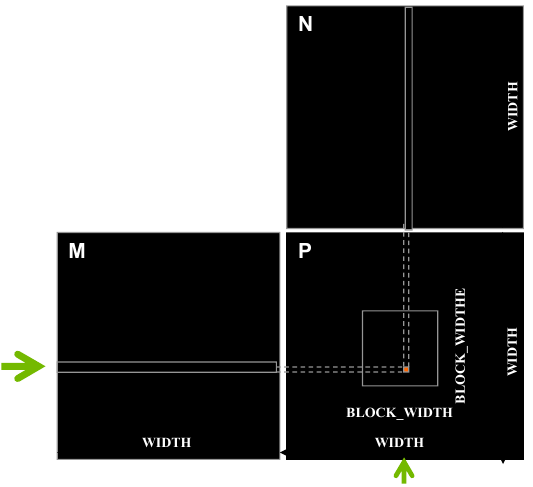
Figure 5: Matrix multiplication (source: NVIDIA DLI).
The output matrix is separated into blocks based on our block size. When writing the kernel, it is necessary to make sure that the index is not out of bounds.
__global__
void matrixMultiplyGPU(float *A, float *B, float *C, int m, int n, int p) {
    int row = blockIdx.y * blockDim.y + threadIdx.y;
    int col = blockIdx.x * blockDim.x + threadIdx.x;
    if (row >= m || col >= p) return;

    float sum = 0.0f;
    for (int k = 0; k < n; k++) {
        sum += A[row * n + k] * B[k * p + col];
    }
    C[row * p + col] = sum;
}
Launch Configuration
The launch configuration is similar to the previous examples. We will launch a 2D grid of blocks, each with a 2D arrangement of threads. The block size will be \(16 \times 16\) and the grid size will be \(m / 16 \times p / 16\). The kernel is launched as follows:
dim3 blockSize(16, 16, 1);
dim3 gridSize((p + blockSize.x - 1) / blockSize.x,
              (m + blockSize.y - 1) / blockSize.y, 1);
matrixMultiplyGPU<<<gridSize, blockSize>>>(A_d, B_d, C_d, m, n, p);
What happens when the output matrix size exceeds the number of blocks per grid and threads per block? If your input is exceeding the maximum grid size, you probably have bigger fish to fry. The largest square grid size that can be launched is \(65536 \times 65536\). The largest square block that can be launched is \(32 \times 32\). This means that your input matrix would need to be larger than \(2097152 \times 2097152\).
What’s Next?
The complexity was slightly increased by considering multidimensional data. Matrices are a prime example of this. The algorithms explored required us to consider multiple input values to compute a single output value. However, the computation did not rely on any thread synchronization, so the task was still simple enough.
Before diving into more complex operations like thread synchronization, was need a better understanding of the GPU’s architecture and memory hierarchy. With this knowledge at our disposal, we can begin to optimize our kernels for maximum performance.