Neural Networks
Linear Models as a Template for Machine Learning
Previously, we studied the Perceptron and saw that while it made for a simple linear classifier, it is severely limited to problems that are already linearly separable. This limitation was resolved by introduding a hidden layer with multiple perceptron units, aptly named Multi-Layer Perceptrons.
In this series, we will explore the more general method of neural networks. We will see that even a network of only two layers can approximate any continuous functional mapping to arbitrary accuracy. Through a discussion about network architectures, activation functions, and backpropagation, we will understand and use neural networks to resolve a large number of both classification and regression tasks.
Before jumping into a definition, consider a simple linear model such as the one discussed in Linear Regression. We can adapt the model to fit all kinds of complex functions through the use of basis functions. Under this variation, it would seem possible to construct a model that fits any function to some arbitrary accuracy. However, this approach suffers greatly from the curse of dimensionality. The more input samples we have, and the more complex they are, the greater then number of parameters required becomes. This was previously discussed when introducing Kernels. Depending on the choice of basis function, the number of parameters required explodes exponentially.
Instead of guessing about which combination of basis functions would result in the best possible model for our particular problem, neural networks are optimized to produce a set of parameters that best fits the training data given a loss function.
Definition
We will take an abstract view of neural networks in which any formulation of a neural network defines a nonlinear mapping from an input space to some output space. This implies that our choice of activation function must be nonlinear. The function we create will be parameterized by some weight matrix \(W\). Thus, any neural network can be simply formulated as
\[ f(\mathbf{x};W). \]
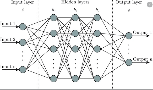
Figure 1: General neural network diagram.
A neural network is in part defined by its layers, the number of nodes in each layer, the choice of activation function, and the choice of loss function.
Each layer has a number of weights equal to the number of input nodes times the number of output nodes. This is commonly represented as a weight matrix \(W\).
The network produces output through the forward pass and computes the gradients with respect to that output in the backwards pass.
Forward Pass
Computing the output is done in what is called the forward pass.
Our neural network function takes in an input \(\mathbf{x} \in \mathbb{R}^D\), where \(D\) is the number of features in our input space. Each output node \(a_j\) in a hidden layer \(h_l\) has a corresponding weight vector \(\mathbf{w}_j^{(l)}\). The intermediate output of a hidden layer \(h_l\) is a linear combination of the weights and the input followed by some nonlinear function. Node \(a_j\) of a hidden layer is computed as
\[ a_j = \sum_{i=1}^d w_{ji}^{(l)} x_{i} + w_{j0}^{(l)}. \]
As with Linear Regression, we will prepend a constant 1 to our input so that the computation is simply
\[ a_{j} = \sum_{i=0}^d w_{ji}^{(i)} x_i = \mathbf{w}_j^T \mathbf{x}. \]
The final output of the hidden layer is \(a_j\) transformed by a nonlinear function \(g\) such that
\[ z_j = g(a_j). \]
We can combine all weight vectors for each hidden layer node into a weight matrix \(W \in \mathbb{R}^{n \times d}\), where \(n\) is the number of nodes in the layer and \(d\) is the number of input features such that
\begin{equation*} W = \begin{bmatrix} \mathbf{w}_1^T\\ \vdots\\ \mathbf{w}_n^T\\ \end{bmatrix}. \end{equation*}
Then the output of the hidden layer can be computed as
\[ \mathbf{a} = W\mathbf{x}. \]
If you instead wanted to separate the bias term, this would be
\[ \mathbf{a} = W\mathbf{x} + \mathbf{b}. \]
Using the notation to specify the individual layer, we can write the output of a full network. Let \(W^{(l)} \in \mathbb{R}^{n_{l} \times n_{l-1}}\) be the weights for layer \(l\) which have \(n_{l-1}\) input connections and \(n_{l}\) output nodes. The activation function for layer \(l\) is given by \(g^{(l)}\).
The complete forward pass of the network is computed by repeating the following step for all layers:
\[ \mathbf{z}^{(l)} = g^{(l)}(\mathbf{a}^{(l-1)}), \]
where
\[ \mathbf{a}^{(l-1)} = W^{(l-1)}\mathbf{z}^{(l-1)} + \mathbf{b}^{(l-1)}. \]
Once all layers have been computed, then the output of the last layer, \(\hat{\mathbf{y}}^{(L)}\) is used as the final output of the model. For training, this is compared with some ground truth label \(\mathbf{y}\) using a loss function \(\mathcal{L}\):
\[ \mathcal{L}(\hat{\mathbf{y}}, \mathbf{y}). \]
XOR Example
Consider the XOR problem. A single Perceptron was unable to solve that problem. However, adding a hidden layer and forming a multi-layer perceptron network allowed for a more complex decision boundary. Consider the network below and produce the output given all combinations of binary input: \(\{(0, 0), (0, 1), (1, 0), (1, 1)\}\).
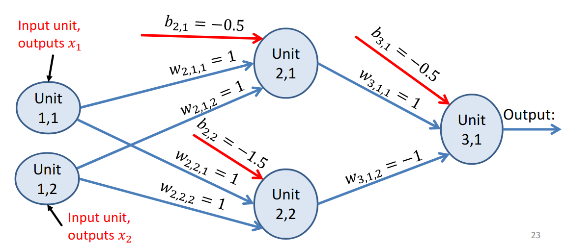
Figure 2: A network with 1 hidden layer that computes XOR. Source: https://athitsos.utasites.cloud/courses/cse4309_fall2021/lectures/09a_neural_networks.pdf
Activation Functions
Sigmoid Function
\[ g(x) = \frac{1}{1 + e^{-x}} \]
The logistic sigmoid function serves two purposes. First, it allows the output of the neuron to be interpreted as a posterior probability. Note that this is not actually a probability. Second, it is a continuous function for which the derivative can be computed:
\[ g’(x) = g(x)(1 - g(x)). \]
Hyperbolic Tangent Function
\[ \tanh x = \frac{e^{x} - e^{-x}}{e^{x} + e^{-x}} \]
The hyperbolic tangent function maps input to a range of \((-1, 1)\).
The derivative is calculated as
\[ \frac{d}{dx} \tanh x = 1 - \tanh^2 x. \]
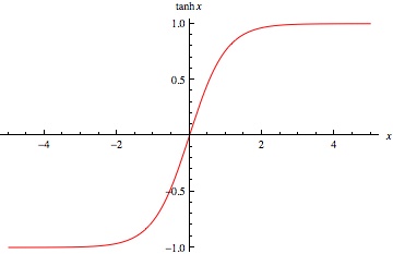
Figure 3: Hyperbolic Tangent Function. Source: Wolfram
Key Terms
- bias
- activation function
- Neurons fire after input reaches some threshold.
- Differential activation functions necessary for backpropagation.
- Multi-class learning
- How long to train?
- Weight decay
- How many layers versus how many nodes per layer?
- Training
- Data split (train/test/val)
Multi-Class Classification
Consider an output layer of a network with \(k\) nodes. Each of these nodes represents a decision node for a one-versus-all classifier. For a classification task, we have to think about whether or not the sum of squares loss function works.
As far as activation functions go, the logistic sigmoid function is a good way to produce some interpretation of probability. If we treat every output node as its own one versus all classifier, then a logistic sigmoid at the end of each one would indicate the “probability” that node \(k\) assigns class \(k\).
How do we formulate this in a neural network?
The number of nodes in the output layer will be \(K\), the number of classes. Since the output of each node produces a value in range \((0, 1)\), we want to construct a target value that works with this. Instead of assigning an integer to each class label (e.g. 1 for class 2, 2 for class 3, etc.), we will encode the target label as a \(K\) dimensional vector. For example, if our class label is for the class 1, then the corresponding target vector will be
\begin{equation*} \mathbf{t} = \begin{bmatrix} 1\\ 0\\ \vdots\\ 0 \end{bmatrix}. \end{equation*}
Since the output of our final layer is also a \(K\) dimensional vector, we can compare the two using some loss function.
Backpropagation
Given a series of linear layers with nonlinear activation functions, how can we update the weights across the entire network?
The short answer is through the chain rule of differentiation. Let’s explore this through an example.
After constructing some series of hidden layers with an arbitrary number of nodes, we will pick an error function that provides a metric of how our network performs on a given regression or classification task. This loss is given by \(\mathcal{L}\).
Neural networks are traditionally trained using gradient descent. The goal is to optimize the weights such that they result in the lowest loss, or error. This is also why our choice of loss function is important.
\[ \mathbf{W}^* = \text{argmin}\frac{1}{n}\sum_{i=1}^n \mathcal{L}(f(\mathbf{x}^{(i)}; \mathbf{W}), \mathbf{y}^{(i)}) \]
We first compute the gradients of the network with respect to the weights and biases. Then, we use those gradients to update our previous values for the weights and biases.
A Simple Example
We will first look at computing these gradients on a smaller network for binary classification with 1 hidden layer and 1 output layer. The loss function is defined using the binary cross-entropy function:
\[ \mathcal{L}(\hat{\mathbf{y}}, \mathbf{y}) = -\mathbf{y}\log \hat{\mathbf{y}} - (1 - \mathbf{y}) \log (1 - \hat{\mathbf{y}}) \]
The network’s output is computed in sequence following
\begin{align*} \mathbf{a}^{(1)} &= W^{(1)}\mathbf{x} + \mathbf{b}^{(1)}\\ \mathbf{z}^{(1)} &= g^{(1)}(\mathbf{a}^{(1)})\\ \mathbf{a}^{(2)} &= W^{(2)}\mathbf{z}^{(1)} + \mathbf{b}^{(2)}\\ \mathbf{z}^{(2)} &= g^{(2)}(\mathbf{a}^{(2)})\\ \end{align*}
The goal is to compute the gradients for all weights and biases:
\[ \frac{d\mathcal{L}}{dW^{(1)}},\quad \frac{d\mathcal{L}}{d\mathbf{b}^{(1)}},\quad \frac{d\mathcal{L}}{dW^{(2)}},\quad \frac{d\mathcal{L}}{d\mathbf{b}^{(2)}}. \]
Starting with the weights of the output layer:
\[ \frac{d\mathcal{L}}{dW^{(2)}} = \frac{d\mathcal{L}}{d\mathbf{z}^{(2)}} \frac{d\mathbf{z}^{(2)}}{d\mathbf{a}^{(2)}} \frac{d\mathbf{a}^{(2)}}{dW^{(2)}}. \]
The first step is to compute the partial gradient of the loss function with respect to its input \(\hat{\mathbf{y}} = \mathbf{z}^{(2)}\):
\[ \frac{d\mathcal{L}}{d\mathbf{z}^{(2)}} = \frac{\mathbf{z}^{(2)} - \mathbf{y}}{\mathbf{z}^{(2)}(1 - \mathbf{z}^{(2)})}. \]
Next, compute the gradient of the last layer’s activation function with respect to its input \(\mathbf{a}^{(2)}\):
\[ \frac{d\mathbf{z}^{(2)}}{d\mathbf{a}^{(2)}} = \mathbf{z}^{(2)}(1 - \mathbf{z}^{(2)}). \]
Finally, we compute \(\frac{d\mathbf{a}^{(2)}}{dW^{(2)}}\): \[ \frac{d\mathbf{a}^{(2)}}{dW^{(2)}} = \mathbf{z}^{(1)}. \]
Putting all of this together yields
\begin{align*} \frac{d\mathcal{L}}{dW^{(2)}} &= \frac{\mathbf{z}^{(2)} - \mathbf{y}}{\mathbf{z}^{(2)}(1 - \mathbf{z}^{(2)})} * \mathbf{z}^{(2)}(1 - \mathbf{z}^{(2)}) * \mathbf{z}^{(1)}\\ &= \mathbf{z}^{(1)} (\mathbf{z}^{(2)} - \mathbf{y}). \end{align*}
Visualizing Neural Networks
Non-Convex Optimization
Optimizing networks with non-linearities produces a non-convex landscape. Depending on our choice of optimization algorithm and initial starting point, the algorithm will most likely get “stuck” in some local minimum. Consider the figure below produced by (Li et al. 2017).
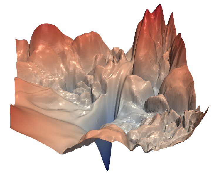
Figure 4: Loss surface of ResNet-56 (Li et al.)