NP-Completeness
Introduction
Most of the algorithms discussed in a typical algorithms course run in polynomial time. This focus is reasonable since algorithms that run worse than polynomial time have little practical use. To simplify this notion: a problem for which a polynomial-time algorithm exists is “easy” and a problem for which no polynomial-time algorithm exists is “hard”. Knowing how to determine whether a problem is easy or hard is extremely useful. If one can identify a hard problem, then an approximate solution may be the best that can be achieved.
One of the most fundamental problems in computer science is the classification of problems into these two categories. These notes provide an introduction to this classification.
P, NP, and NP-Complete
We start with three classes of algorithms:
- Polynomial-time
- NP (nondeterministic polynomial time)
- NP-complete
Problems in P are those solvable in polynomial time. This means any constant \(k\) such that the running time is \(O(n^k)\).
The class NP is a superset of P. These are problems that can be verified in polynomial time. This means that if someone gives you a solution to the problem, you can verify that it is correct in polynomial time. This is different from solving the problem in polynomial time. Problems in NP can be solved in nondeterministic polynomial time. However, such a model of computation does not exist in the real world.
There is also a class of problems labeled NP-Hard. These are problems that cannot be solved in polynomial time, nor can they be verified in polynomial times. Basically, they are not decision problems. This class includes certain optimization problems and the classic Halting problem.
NP-Complete problems are problems in NP that are as hard as any other problem in NP. This means that if you can solve an NP-Complete problem in polynomial time, you can solve any problem in NP in polynomial time. This is why NP-Complete problems are so important.
Verifying a Solution
As long as we can come up with a verification algorithm for a problem in polynomial time, we can say that the problem is in \(NP\). This is true even if we later find a polynomial-time algorithm for the problem.
Proving that a problem is NP-Complete
Proving that a problem belongs to either NP or NPC is difficult the first time you do it. Luckily, now that problems have been proven to be NP-Complete, you can use these problems to prove that other problems are NP-Complete. Informally, a problem \(X\) is NP-Hard if it is at least as hard as any problem in NP. If we can reduce every problem \(Y \in NP\) to \(X\) in polynomial time, then \(X\) is NP-Hard. If \(X\) is also in NP, then \(X\) is NP-Complete.
Optimization versus decision problems
Many problems are framed as optimization problems. Given some criteria, the goal is to find the best solution according to that criteria. For the shortest path problem, the algorithm finds a path between two vertices in the fewest number of edges. One can intuit that this is a slightly harder problem than that of determining if a path exists using only \(k\) edges. This latter problem is a decision problem.
The reason this is worth talking about is that decision problems are often easier to come up with than optimization problems. If one can provide that a decision problem is hard, then its optimization problem is also hard.
Reducing one problem to another
A common strategy for relating two problems is to reduce one to the other. For example, if problem \(B\) runs in polynomial time, and we can reduce problem \(A\) to problem \(B\) in polynomial time, then problem \(A\) is also in P. This is because we can solve \(A\) by reducing it to \(B\) and then solving \(B\) in polynomial time.
Reductions
The main idea behind reductions is to first show that a problem is NP-Complete. This first proof was done by Cook in 1971. With a problem proven to be NP-Complete, one can then show that other problems are NP-Complete by reducing them to the first problem. This method is far simpler than the original proof and provides a convenient process for proving that a problem is NP-Complete. The process is based on the following lemma.
Lemma 34.8
If \(L\) is a language such that \(L’ \leq_p L\) for some \(L’ \in \text{NPC}\), then \(L\) is NP-hard. If, in addition, we have \(L \in \text{NP}\), then \(L\) is NP-Complete.
Circuit Satisfiability
- What is this problem?
- Why is it important?
- How is it related to NP-Completeness?
Given a boolean combinatorial circuit, is it satisfiable. That is, is there an assignment of values to the inputs that makes the output true?
This problem is in the class NP. To prove this, we only need to show that given an assignment of values to the inputs, we can verify that the output is true in polynomial time. For a given circuit, we can verify that the output is true by following the circuit from the inputs to the outputs.
Proving that it is NP-Complete is much more difficult, so a brief overview is provided here. Let \(A\) be any problem in \(NP\). Since any problem in \(NP\) has a polynomial-time verification algorithm, we can construct a boolean circuit that simulates this algorithm. This circuit will have a single output that is true if and only if the input is a valid solution to the problem. This circuit is satisfiable if and only if the input is a valid solution to the problem. Therefore, the circuit satisfiability problem is NP-Complete.
Example: Exercise 34.3-1
Verify that the given circuit is unsatisfiable.
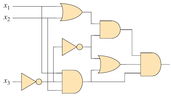
Figure 1: Figure 34.8 from (Cormen et al. 2022).
For reference, here are definitions for each of the gates listed in the figure.
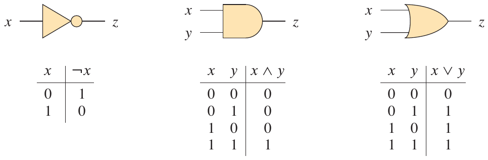
Figure 2: Definitions for the gates in the circuit from Figure 34.7 (Cormen et al. 2022).
How can we prove this circuit is unsatisfiable?
The easiest way to do this is to code it up and brute force it.
The satisfiability problem was the first problem proved to be NP-Complete by the Cook-Levin theorem. Cormen et al. describe a summarized proof in section 34.3 (Cormen et al. 2022). Michael Sipser’s book on the theory of computation offers a more detailed sketch of the proof (Sipser 2012). You can also watch his lecture on the Cook-Levin theorem from MIT.
The basic idea of the proof is as follows. For any problem in NP, there exists some machine that can verify solutions in polynomial time. Cook’s proof involves simulating this machine with a Boolean formula. The idea is to encode the computation of the machine as a sequence of logical operations that can be expressed as a Boolean formula. Since the boolean formula is satisfiable if and only if the machine accepts the input, the satisfiability problem is NP-Complete.
Formula Satisfiability
- Satisfiability (SAT) is NP-Hard.
- Can show that CIRCUIT-SAT \(\leq_p\) SAT.
- Then show that SAT \(\leq_p\) 3SAT.
An instance of the formula satisfiability (SAT) problem is a boolean formula \(\phi\) with
- \(n\) variables \(x_1, x_2, \ldots, x_n\)
- \(m\) clauses \(C_1, C_2, \ldots, C_m\)
For example, the formula
\[ \phi = (x_1 \lor x_2) \land (\lnot x_1 \lor x_3) \land (x_2 \lor x_3) \]
has the satisfying assignment \(x_1 = 1, x_2 = 0, x_3 = 1\).
SAT belongs to NP
Showing that SAT is in NP is straightforward. Given a boolean formula \(\phi\) and an assignment of values to the variables, one can verify that the formula is satisfied in polynomial time. This is enough to show that SAT is in NP.
CIRCUIT-SAT \(\leq_p\) SAT
If we can reduce an instance of CIRCUIT-SAT, which is known to be NP-Complete, to SAT, then SAT is also NP-Complete. This proof is by contradiction: assume that SAT is not NP-Complete. Then, CIRCUIT-SAT is not NP-Complete. But we know that CIRCUIT-SAT is NP-Complete, so this is a contradiction.
The reduction starts by introducing a variable for each wire and a clause for each gate, as seen below.
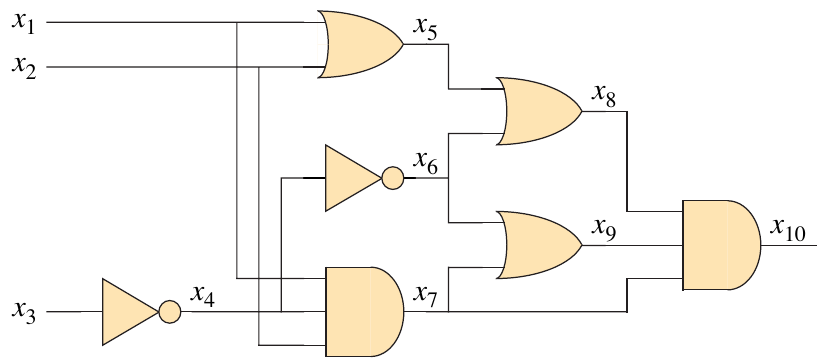
The reduction algorithm produces a formula for each gate in terms of an “if and only if” statement.
\begin{align*} \phi = x_{10} &\land (x_4 \leftrightarrow \lnot x_3)\\ &\land (x_5 \leftrightarrow (x_1 \lor x_2))\\ &\land (x_6 \leftrightarrow \lnot x_4)\\ &\land (x_7 \leftrightarrow (x_1 \land x_2 \land x_4))\\ &\land (x_8 \leftrightarrow (x_5 \lor x_6))\\ &\land (x_9 \leftrightarrow (x_6 \lor x_7))\\ &\land (x_{10} \leftrightarrow (x_6 \land x_8 \land x_9))\\ \end{align*}
A simpler explanation for this reduction is that a circuit can be represented as a boolean formula. This formula can be solved by the SAT algorithm.
3SAT
The 3SAT problem is a special case of SAT where each clause has exactly three literals. This problem is also NP-Complete. Many problems can be reduced to 3SAT, which is why it is so important.
Definition
An instance of 3SAT is a boolean formula \(\phi\) with
- \(n\) literals \(x_1, x_2, \ldots, x_n\)
- \(m\) clauses \(C_1, C_2, \ldots, C_m\)
Each clause has exactly three literals and is in conjunctive normal form (CNF), which means it is expressed as an AND of clauses. For example, the formula
\[ \phi = (x_1 \lor x_2 \lor x_3) \land (\lnot x_1 \lor x_2 \lor x_3) \land (x_1 \lor \lnot x_2 \lor x_3) \]
is a 3SAT formula.
3SAT is NP-Complete
The 3SAT problem is NP-Complete. This can be shown by reducing SAT to 3SAT. A thorough proof is provided in the textbook (Cormen et al. 2022).
Clique Problem
A clique is a complete subgraph of an undirected graph \(G\). That is, a clique is a set of vertices such that every pair of vertices is connected by an edge. The clique problem is to find the largest clique in a graph.
\[ \text{CLIQUE} = \{ \langle G, k \rangle \mid G \text{ has a clique of size } k \} \]
Clique is in NP
Let’s say you have access to a clique of size \(k\). You can verify that this is a clique in polynomial time by checking that every pair of vertices is connected by an edge. That is, for each pair \(u, v \in V’\), the edge \((u, v)\) is in \(E\), where \(V’\) is the set of vertices in the clique.
Thus, we have a polynomial-time verification algorithm for the clique problem, so it is in NP.
Clique is NP-Complete
Knowing that 3SAT is NP-Complete, we can reduce 3SAT to the clique problem. The reduction may not be intuitive as a boolean formula seems to have no relation to a graph.
Let \(\phi = C_1 \land C_2 \land \ldots \land C_m\) be a 3SAT formula with \(n\) variables. We construct a graph \(G\) with \(3n\) vertices. Each \(C_r\) has three literals, \(l_1^r, l_2^r, l_3^r\).
To construct the graph, we create a triplet of vertices \(v_1^r, v_2^r, v_3^r\) for each clause \(C_r\) such that there is no edge connecting any two vertices in the same triplet. There is an edge \((v_i^r, v_j^s) \in E\) if
- \(v_i^r\) and \(v_j^s\) are in different triplets
- \(l_i^r\) and \(l_j^s\) are not negations of each other
One such formula that we can convert is
\[ \phi = (x_1 \lor \lnot x_2 \lor \lnot x_3) \land (\lnot x_1 \lor x_2 \lor x_3) \land (x_1 \lor x_2 \lor x_3). \]
The resulting graph is shown below.
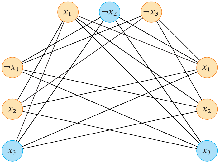
Figure 3: Graph constructed from the 3SAT formula (phi) (Cormen et al. 2022).
If a satisfying assignment exists for \(\phi\), then each \(C_r\) has at least one literal that is true. Consider the corresponding vertices in the graph for a satisfying assignment. Since there is at least one true literal in each clause, there is at least one edge between the corresponding vertices. Thus, a reduction from 3SAT to the clique problem is possible.
How does this show that Clique is NP-Complete?
It is true that this example shows a very specialized graph. However, this is enough to show that the problem is NPC. If there were a polynomial time solution for Clique on a general graph \(G\), then surely it would work for a specialized graph as well.
If it could solve this one, then the corresponding 3SAT formula would be solvable as well. This is a contradiction, so the Clique problem is NP-Complete.
Vertex Cover Problem
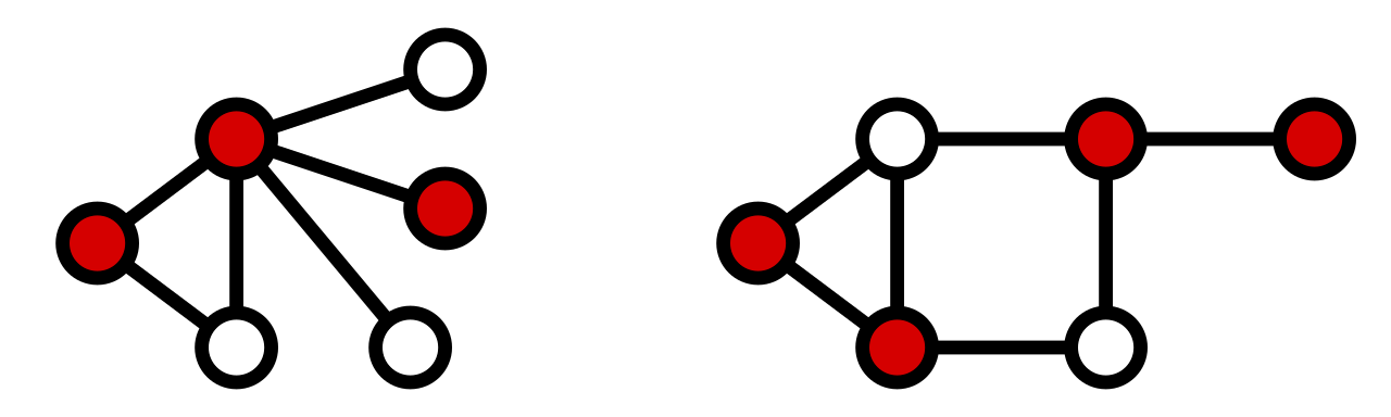
Figure 4: Vertex cover examples (Wikipedia).
The vertex cover problem is to find the smallest set of vertices such that every edge in the graph is incident to at least one vertex in the set. More formally, a vertex cover of a graph \(G\) is a set \(V’ \subseteq V\) such that for every edge \((u, v) \in E\), either \(u \in V’\) or \(v \in V’\).
Vertex Cover is in NP
Given a set of vertices \(V’\), one can verify that it is a vertex cover in polynomial time by checking that every edge is incident to at least one vertex in the set. This is a polynomial-time verification algorithm, so the vertex cover problem is in NP.
Vertex Cover is NP-Complete
We can show that the vertex cover problem is NP-Complete by reducing it to an instance of the clique problem. For this, we need to introduce the definition of a graph complement. Given a graph \(G = (V, E)\), the complement of \(G\) is the graph \(\overline{G} = (V, E’)\) where \(E’ = \{ (u, v) \mid u, v \in V \text{ and } (u, v) \notin E \}\). Basically, \(\overline{G}\) has all the edges that \(G\) does not have.
Let \(G\) contain a clique \(V’ \subseteq V\), where \(|V’| = k\). Then \(V - V’\) is a vertex cover of \(\overline{G}\). If \((u, v) \in \overline{E}\), but is not in \(E\), then at least one of \(u\) or \(v\) is not in \(V’\).
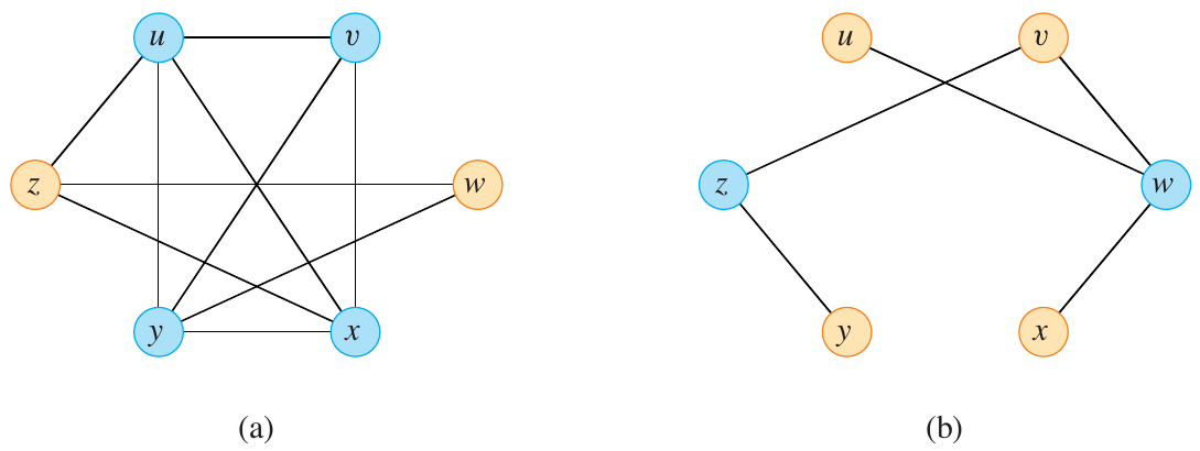
Figure 5: Graph (G) and its complement (overline{G}) (Cormen et al. 2022).
In the example above, any edge in \(\overline{G}\) has at least one vertex that is not in \(G\). On the same edge, at least one is in \(V - V’\), implying that \((u, v)\) is covered by \(V - V’\). Thus, a reduction from the clique problem to the vertex cover problem is possible.