Object Detection
Papers
Evaluating Object Detection Methods
Object detection algorithms are evaluated using the mean of Average Precision (mAP) across all classes in the dataset.
Precision and recall are computed from the predictions and the ground truth. A sample and the model’s prediction can either be positive or negative when it comes to classification. Either it belongs to a class or it does not. The table below summarizes the outcomes between the model’s prediction and the true underlying class.
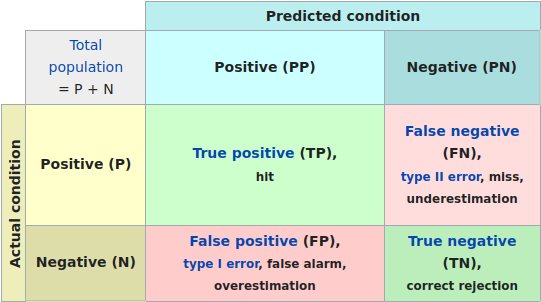
Figure 1: Confusion matrix (Source: Wikipedia)
Object detection algorithms are evaluated using the mean of Average Precision (mAP) across all classes in the dataset.
Precision and recall are computed from the predictions and the ground truth. A sample and the model’s prediction can either be positive or negative when it comes to classification. Either it belongs to a class or it does not. The table below summarizes the outcomes between the model’s prediction and the true underlying class.
Precision
\[ \frac{TP}{TP + FP} \]
Recall
\[ \frac{TP}{TP + FN} \]
Object detection models predict a bounding box for a given class. A correct bounding box can be identified as one that has an Intersection-over-Union (IoU) score of > 0.5.
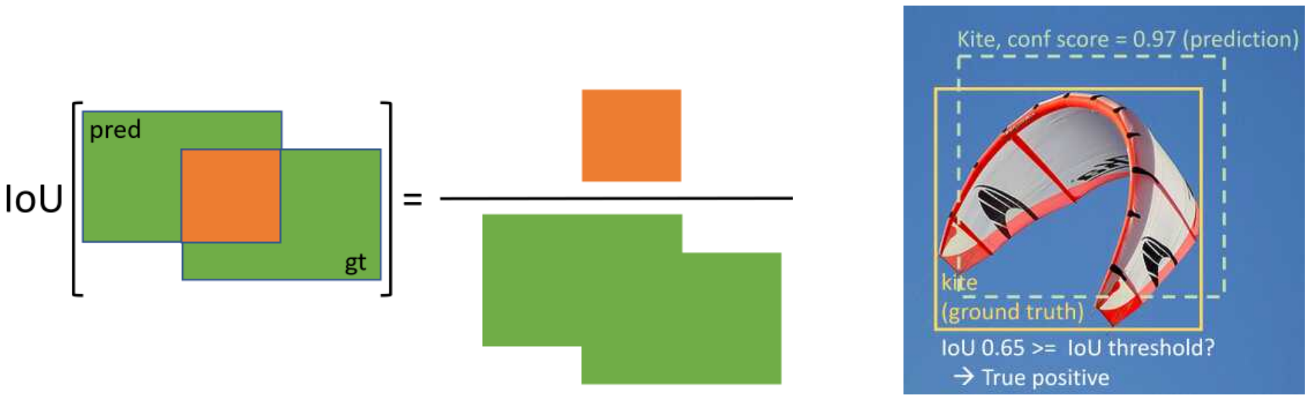
Figure 2: IoU Visualization (Szeliski 2021)
If you were to plot the precision versus recall of a single class, the area under the curve would be the average precision.
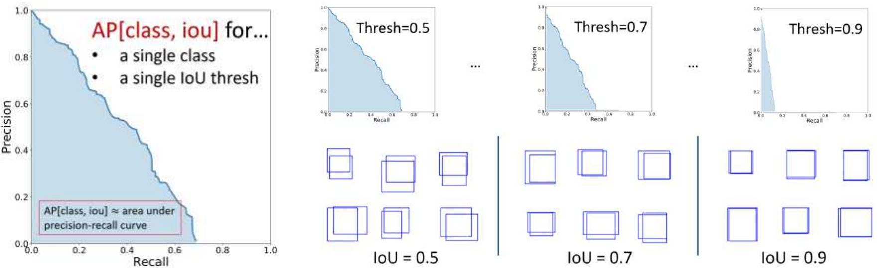
Figure 3: Average Precision Curves (Girshick, 2020)
The curve implicitly represents varying probability thresholds! As recall increases, precision will generally decrease. This reflects the fact that a model that recalls all input samples as a particular class will sure be misclassifying them. Keep in mind that recall by itself is not a measure of correctness. Ideally, the curve will be closer to the top right of the graph, indicating high precision and recall.
Datasets
An Incomplete History of Deep-Learning-based Object Detection
Rich Feature Hierarchies for Accuracy Object Detection and Semantic Segmentation (Girshick et al. 2014)
The last decade of progress on various visual recognition tasks has been based considerably on the use of SIFT and HOG (Girshick et al. 2014).
This is one of the earliest papers to leverage deep learning for object detection. The overall approach is a piecewise one, where the CNN is only used for classification.
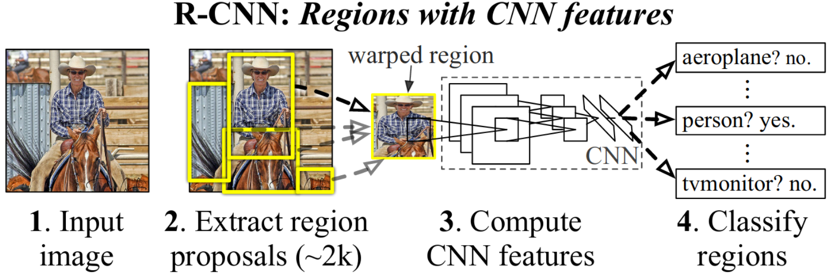
Figure 4: System overview of the R-CNN approach (Girshick et al. 2014)
Key Insights
- Increased mean average precision (mAP) by more than 30% on VOC 2012.
- Candidate regions are generated using Selective Search (Uijlings et al. 2013).
- CNNs are used to perform object classification for each region proposal.
- Employs bounding box regression to refine the predicted bounding boxes.
- “…when labeled training data is scarce, supervised pre-training for an auxiliary task, followed by domain-specific fine-tuning, yields a significant performance boost.”
Region Proposals
The Selective Search algorithm is used to generate region proposals. The algorithm is based on hierarchical grouping of superpixels. Given an input image, approximately 2000 region proposals are generated. Each region proposal is a rectangular bounding box that encloses a region of interest. Since the bounding boxes are not square, the prposals are warped to a fixed size before being fed into the CNN.
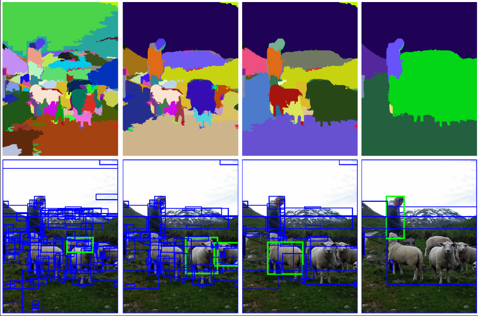
Figure 5: Selective Search region proposals (Uijlings et al. 2013).
Feature Extraction
Each warped image is passed through a CNN backbone pre-trained on ImageNet. The output is a 4096-dimensional feature vector. In the context of today’s methods, this certainly does not seem like a very sophisticated approach. Given the context of the time, this was a significant improvement over the SIFT and HOG features that were previously used. The other benefit is that the CNN can be fine-tuned on the target dataset, if desired.
Classification
The feature vectors from the CNN are used as input to a linear SVM for classification. The SVM is trained to classify the region proposals into one of the classes in the dataset. As stated before, this really is a piecewise solution. It is also very slow, as each region proposal must be passed through the CNN and SVM.
Training
The CNN and SVM both need to be trained. The CNN is first pre-trained on ImageNet, but it still needs to be fine-tuned on the target dataset. Not only is the target dataset out of domain, but the images themselves are warped. The authors do admit that it is reasonable to simply use the output of the softmax layer for classification in stead of training an SVM. In their experiments, they found that the SVM provided a slight improvement in performance.
Inference
Given roughly 2000 region proposals, how is a final prediction made? For each class, non-maximum suppression is applied to the region proposals. A region is rejected if it has an IoU overlap with a higher scoring region above a certain threshold.
Fast R-CNN (Girshick 2015)
Published roughly a year after the original R-CNN paper, Fast R-CNN addresses many of the shortcomings and ineffeciencies of the original approach. The main innovation is the introduction of the Region of Interest (RoI) pooling layer. This layer allows the CNN to be applied to the entire image, rather than to each region proposal individually.
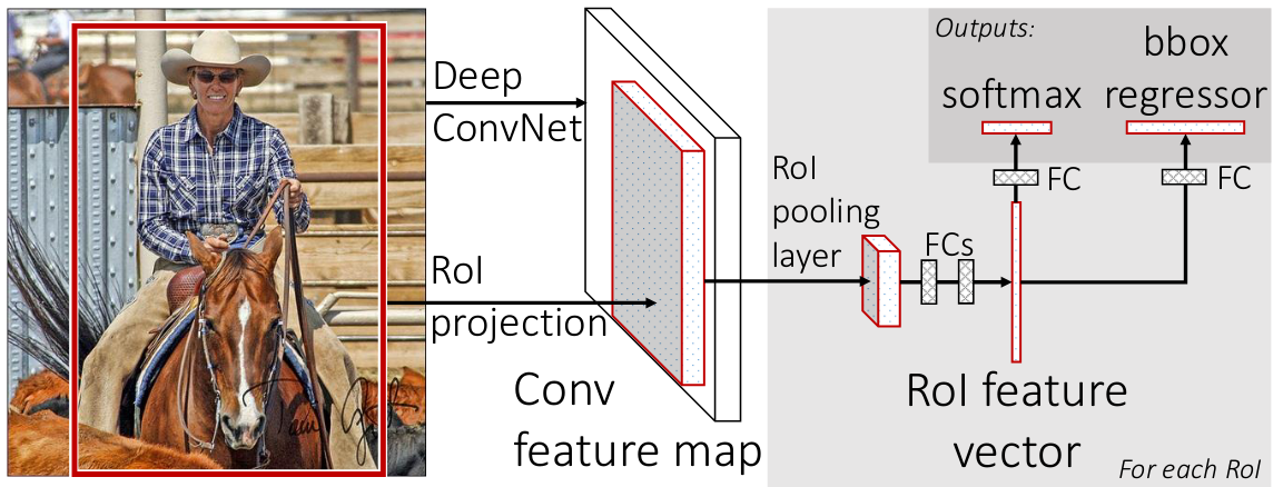
Figure 6: System overview of Fast R-CNN (Girshick 2015)
Key Insights
- Single-stage training joinly optimizes a softmax classifier and bounding box regressor.
- RoI pooling layer allows the CNN to be applied to the entire image.
- Object proposals are still provided by Selective Search, but only a single forward pass is needed to extract features and make predictions.
RoI Pooling
Given an input image, a feature extracting CNN produces a feature map. For each region proposal the RoI pooling layer extracts a feature vector directly from the feature map. The feature vector is passed through a fully connected network to produce a class score and bounding box regression.
A region proposal is defined by a four-tuple \((r, c, h, w)\) defining the top-left corner \((r, c)\) and the height and width \((h, w)\) of the region. The RoI pooling layer divides the window into a \(H \times W\) grid of sub-windows, where \(H\) and \(W\) are hyperparameters. A max pooling operation is applied to each sub-window to produce a fixed-size output.
For more details on exactly how RoI pooling is implemented, see Kemal Erdem’s excellent blogpost.
Training
Three different CNN backbones were tested. The last max pooling layer is replaced with the RoI pooling layer. From there, the two branches of the network are added: a softmax classifier and a bounding box regressor. The softmax classifier is trained to classify the region proposals into one of the classes in the dataset. The bounding box regressor is trained to refine the predicted bounding boxes.
Another key efficiency improvement comes from hierarchical sampling during training. Since the RoI pooling layer allows the CNN to be applied to the entire image, the same feature map can be used for multiple region proposals. This is in contrast to the original R-CNN approach, where each region proposal was passed through the CNN individually. When training, the authors sample a mini-batch of \(N\) images and \(R\) regions, yielding \(R / N\) RoIs from each image.
Results
This work achieved state-of-the-art results on VOC 2007 (70.0), 2010 (68.8), and 2012 (68.4). Additionally, the model was able to run at about 5 frames per second on a GPU.
Faster R-CNN (Ren et al. 2017)
Fast R-CNN improved on many of the glaring issues presented in the original R-CNN paper. One major bottleneck left was the Selective Search algorithm used to generate region proposals. In the third iteration, Faster R-CNN, the authors introduce the Region Proposal Network (RPN) to replace slower region proposal methods.
Key Insights
- Region Proposal Network (RPN) generates region proposals.
- RPN is a fully convolutional network that shares features with the object detection network.
- Anchor boxes of varying aspect ratios are used to predict region proposals.
Region Proposal Network
The RPN uses a sliding window approach to generate region proposals. Instead of using a separate CNN, it leverages the feature maps generated by a backbone CNN such as VGG or ResNet.
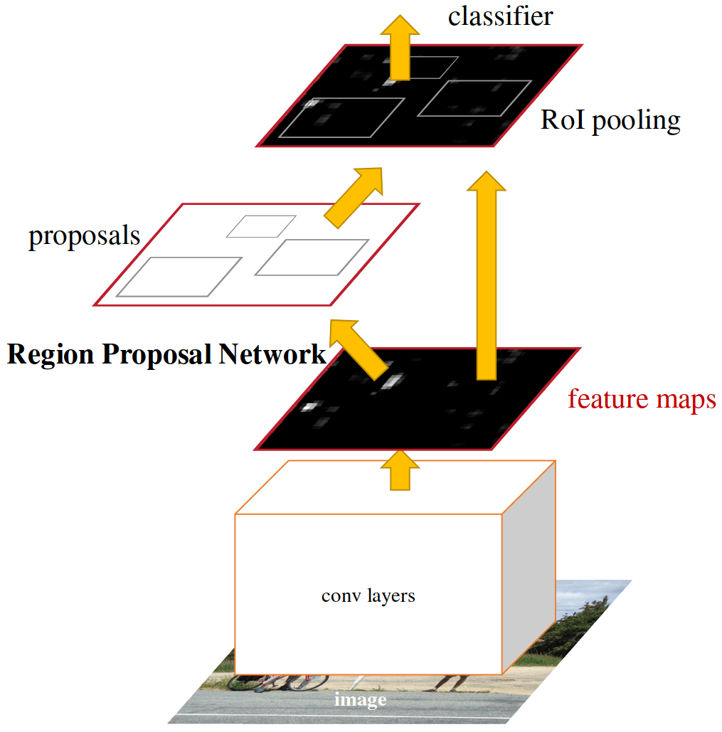
Figure 7: Region Proposal Network (RPN) (Ren et al. 2017)
The RPN produces a feature vector for each sliding window, which is fed into a bounding box regressor and classifier. For each of these sliding windows, \(k\) anchor boxes are generated. In their experiments, they generate 9 anchors based on 3 scales and 3 aspect ratios.
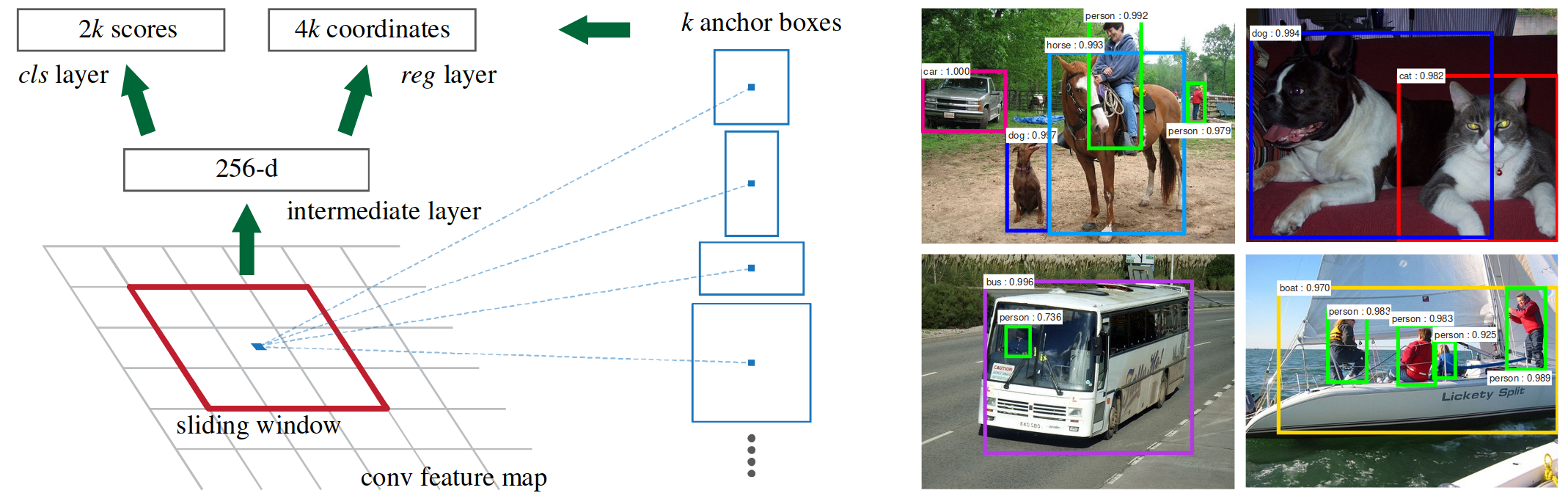
Figure 8: Anchor boxes (Ren et al. 2017)
Why use anchor boxes instead of directly predicting bounding boxes? The authors argue that using anchor boxes simplifies the problem. It adds translation invariance: if an object is translated, the proposal should translate accordingly. This approach is also more cost-efficient. Consider an input image for which multiple scales of bounding boxes are generated. To generate multiple scales, the image would need to be resized and passed through the network multiple times. With anchor boxes, the network only needs to be run once.
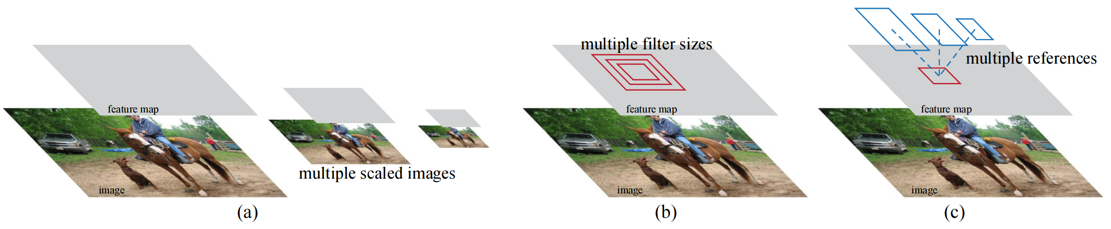
Figure 9: Different schemes for addressing multiple scales and sizes (Ren et al. 2017).
Results
Faster R-CNN achieved state-of-the-art results on VOC 2007 (73.2) and 2012 (70.4). These scores increase to 78.8 and 75.9 when using the COCO dataset. Additionally, they evaluate on MS COCO, achieving a mAP@.5 of 42.7, meaning that the model is able to detect 42.7% of the objects in the dataset with an IoU of 0.5 or greater. This score goes down to 21.9% when the IoU threshold is expanded in the range of 0.5 to 0.95.
You Only Look Once
You Only Look Once (YOLO) is a single-stage object detection algorithm that is able to predict multiple bounding boxes and class probabilities in a single forward pass (Redmon et al. 2016). Since 2016, it has benefitted from many improvements, some documented by peer-reviewed papers and others by the community. For a recent survey of YOLO and its variants, see (Terven, Córdova-Esparza, and Romero-González 2023).
YOLOv1 (Redmon et al. 2016)
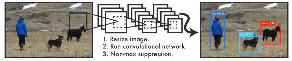
Figure 10: YOLOv1 Overview (Redmon et al. 2016)
The original YOLO method works by dividing an input image into a \(S \times S\) grid. Each grid cell predicts \(B\) bounding boxes and confidence scores for each box, along with \(C\) class probabilities.
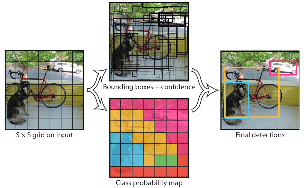
Figure 11: The Model (Redmon et al. 2016).
During training, only one predictor should be responsible for each object. This is enforced by assigning a predictor to an object based on the highest IoU with the ground truth. For inference, the model outputs bounding boxes with a confidence score greater than a threshold. The entire model is trained using a multi-part loss function that includes terms for objectness, classification, and bounding box regression.
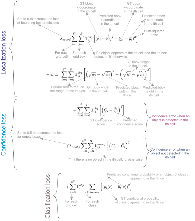
Figure 12: Annotated description of YOLO loss (Terven, Córdova-Esparza, and Romero-González 2023).
YOLOv1 was evaluated on the VOC 2007 dataset, achieving a mAP of 63.4. The model was able to run at 45 frames per second on a GPU.
YOLOv2: Better, Faster, and Stronger (Redmon and Farhadi 2016)
YOLOv2 was publised at CVPR 2017 and introduced several key improvements over YOLOv1.
- Batch normalization acts as a regularizer to reduce overfitting during training.
- Fully convolutional. All dense layers are replaced with convolutional layers.
- Following Faster R-CNN, YOLOv2 uses anchor boxes to predict bounding boxes.
- A predetermined set of anchor box sizes are computed using k-means clustering on the training data.
- The model was trained to be robust to varying sizes via multi-scale training, where the input image is randomly resized during training.
- Multi-task Learning. The network is pre-trained on ImageNet, where no object detection labels are used. In the event that an input sample does not contain a bounding box annotation, the model is trained to predict the background class.
YOLOv2 achieved a 73.4% mAP on VOC 2012, beating Faster R-CNN.
YOLOv3 (Redmon and Farhadi 2018)
The third improvement to YOLO was not published at a major conference, but was released on arXiv. The main improvement is a deeper 53-layer backbone network with residual connections. The new method also supports multi-scale predictions by predicting three boxes at three different scales. The same anchor box computation via k-means is done in this work, with the number of priors being expanded to support three different scales.
YOLOv4 and beyond
The remaining iterations were developed by other members of the community and introduce several key improvements while maintaining the spirit and goals of the original paper. For more information, see the informative survey paper by (Terven, Córdova-Esparza, and Romero-González 2023).