Optical Flow
Introduction
Optical flow refers to the apparent motion in a 2D image. Optical flow methods estimate a motion field, which refers to the true motion of objects in 3D. If a fixed camera records a video of someone walking from the left side of the screen to the right, a difference of two consecutive frames reveals much about the apparent motion.
Many different approaches to optical flow have been proposed from classical, algorithmic methods to deep learning-based methods. These notes will focus on the definition and classical methods, leaving the rest for future lectures.
Motion Features
Motion features are used a wide variety of tasks from compression, image segmentation, tracking, detection, video de-noising, and more. For example, human activity recognition methods can leverage motion features to identify complex actions. Along with traditional image-based features,
Consider a sphere with Lambertian reflectance.
If the sphere is rotated:
- What does the motion field look like?
- What does the optical flow look like?
If, instead, a point light is rotated around the sphere:
- What does the motion field look like?
- What does the optical flow look like?
It is also possible to infer relative depth from video. As the sphere moves towards the camera, its apparent size will become larger. If we were to analyze the optical flow of such a sequence, we would see that the flow is radial as the sphere, projected as a circle, grows.
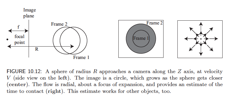
Figure 1: From “Computer Vision - A Modern Approach” by Forsyth and Ponce
At \(t=1\), the radius of the circle is given as \(R\). At \(t=2\), the radius is \(r = f\frac{R}{Z}\), where \(f\) is some function of the motion and \(Z\) is the distance between the sphere and the camera. From this, we can also compute the speed at which the sphere is travelling towards the camera as \(V=\frac{dZ}{dt}\). The apparent rate of growth as observed by the camera is \(\frac{dr}{dt} = -f\frac{RV}{Z^2}\). We can also determine the time to contact with the camera as \(-\frac{Z}{V}\).
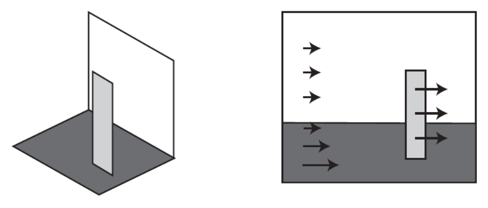
Figure 2: Optical flow on different parts of the image as observed from a moving camera whose direction of focus is perpendicular to the white plane. Source: “Computer Vision - A Modern Approach” by Forsyth and Ponce
In the figure above, the observer is moving at a constant rate to the left. The points in the image appear to translate towards the right edge of the frame. Points that are close to the camera appear to move faster than those that are farther away. This can be used to estimate the apparent depth between objects in a scene.
Computing Optical Flow
A popular assumption for optical flow, as discussed in (Horn and Schunck 1980), is that of brightness constancy. A local feature has the same image intensity in one frame as it does in the subsequent frame.
\[ I(x + u, y + v, t + 1) = I(x, y, t) \]
The Aperture Problem
Consider a small window in an image. As the subject in the image moves, the window will only capture the motion in the direction of the gradient. This is known as the aperture problem.
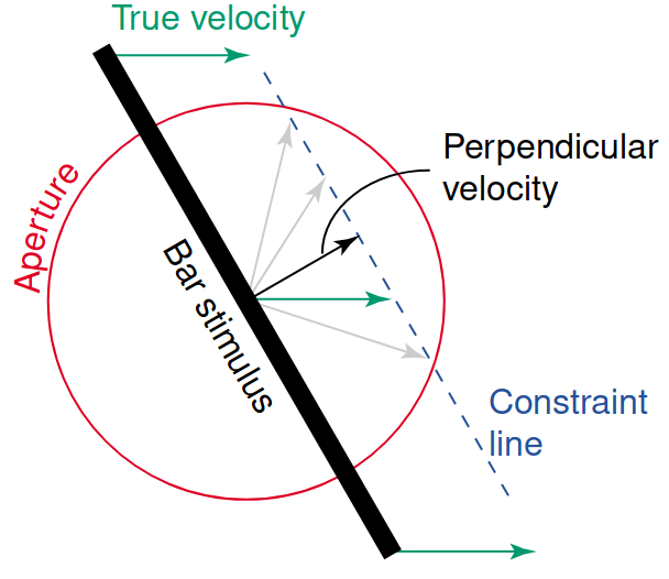
Figure 3: The aperture problem (Murakami 2004).
The problem is that only one direction of motion can be established, but there are many possible directions of motion. Mathematically, the system is underconstrained because there are two unknowns (\(u\) and \(v\)) for each pixel.
Local Constancy and Smoothness
One way to address the aperture problem is to assume that the motion is constant within a local neighborhood (Lucas and Kanade 1980). Given a window of size \(n \times n\), we have \(n^2\) equations for each pixel. This is a more constrained system and can be solved using the normal equations.
An additional assumption is that the motion is smooth across the image. This is known as the smoothness assumption. The energy function is then modified to include a term that penalizes the difference in motion between neighboring pixels (Horn and Schunck 1980).
Given these two constraints, we can formulate an objective function. First, the objective function assuming brightness constancy is given by
\[ E_D(\mathbf{u}, \mathbf{v}) = \sum_{s}(I(x_s + u_s, y_s + v_s, t + 1) - I(x, y, t))^2. \]
Adding in the assumption of uniform motion in a local region yields the term
\[ E_S(\mathbf{u}, \mathbf{v}) = \sum_{n\in G(s)}(u_s - u_n)^2 + \sum_{n \in G(s)}(v_s - v_n)^2. \]
Putting these together, with a weighting term, yields
\[ E(\mathbf{u}, \mathbf{v}) = E_D + \lambda E_S. \]
This energy function \(E_D\) is minimized by differentiating and setting the equation to 0:
\[ I_x u + I_y v + I_t = 0. \]
To be more specific, a Taylor series approximation of the original difference equation is used to derive the above equation. The Taylor series is truncated at the first order since the assumption is that the motion is small; the higher order terms are negligible. Taking the first order approximation allows us to compute the flow at sub-pixel accuracy. More importantly, it allows us to frame the problem as a system of linear equations. The entire energy to be minimized is then
\[ E_D(\mathbf{u}, \mathbf{v}) = \sum_{s}(I_{x,s}u_s + I_{y,s}v_s + I_{t,s})^2 + \lambda \sum_{n\in G(s)}(u_s - u_n)^2 + \sum_{n \in G(s)}(v_s - v_n)^2. \]
Differentiating this and setting to 0 yields two equations in \(u\) and \(v\):
\begin{align*} \sum_s{(I_{x,s}^2 u_s + I_{x,s}I_{y,s}v_s + I_{x,s}I_{t,s}) + \lambda \sum_{n \in G(s)}(u_s - u_n)} &= 0\\ \sum_s{(I_{x,s}I_{y,s} u_s + I_{y,s}^2v_s + I_{y,s}I_{t,s}) + \lambda \sum_{n \in G(s)}(v_s - v_n)} &= 0\\ \end{align*}
Note that this is computed for every pixel in the image. This system is no longer underspecified because of the assumption that neighbors will exhibit the same flow. We now have 5 equations per pixel. In more recent works, larger neighborhood grids (\(5 \times 5\)) are used. Then, we have 25 equations per pixel. Since this is a system of linear equations, it could be computed directly using the normal equations.
However, Horn and Schunck did not have very fast computers in 1981. So, they introduced an iterative solution (Horn and Schunck 1980).
Assumptions of Small Motion
One of the core assumptions in early formulations of optical flow is that motion is very small (<1 pixel). In reality, some objects may move over 100 pixels within a single frame. A simple solution to this problem was proposed by Bergen et al. in 1992 (Bergen et al., n.d.). By creating an image pyramid over several resolutions, the assumption of small motion at each scale is still reasonable.
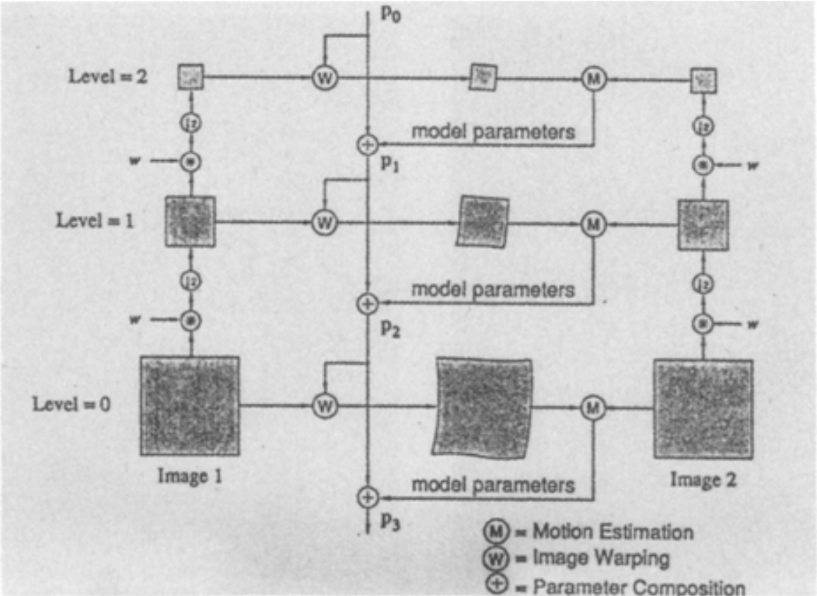
Figure 4: Hierarchical motion estimation (Bergen et al., n.d.)
At one scale, the warping parameters are estimated. Next, they are used to warp the image to match the one at \(t-1\). The warped image and true image at \(t-1\) are compared to refine the parameters. The refined parameters are then sent to the next scale layer.
Applications
- Features for tracking
- Segmentation
- Optical mouse (used in early mice)
- Image stabilization
- Video compression
- Datasets (Sintel)
- … and more