Optimization for Deep Learning
Resources
- https://ruder.io/optimizing-gradient-descent/
- https://www.deeplearningbook.org/contents/optimization.html
Introduction
empirical risk minimization - minimizing over an empirical distribution. Differs from risk minimization which is minimizing over the true distribution. We typically do not know the true distribution.
Complex models are able to memorize the dataset.
In many applications for training, what we want to optimize is different from what we actually optimize since we need to have useful derivatives for gradient descent. For example, the 0-1 loss
\begin{equation*} L(i, j) = \begin{cases} 0 \qquad i = j \\ 1 \qquad i \ne j \end{cases} \qquad i,j \in M \end{equation*}
is what we would really want to minimize for classification tasks. In practice we use something like Cross Entropy Loss. As pointed out by (Goodfellow et al.), there are sometimes advantages with using surrogate loss functions. A 0-1 loss may eventually fit the training set with 100% accuracy. At this point, no further optimization could take place as the error would be 0. With losses like negative log likelihood, optimization could continue which may result in increasing the margin between classes.
Larger batch sizes provide a more accurate estimate of the gradient.
Randomly selecting samples is crucial for learning. Datasets may be arranged in such a strong bias is present. Shuffling once isn’t enough because the data is biased after the first iteration. We could only get around this if we had the true distribution to generate new samples.
If our training set is extremely large, we may converge to a solution without ever having gone through all samples. Typically, models are able to train on multiple passes of the dataset to increase their generalization error. Each subsequent pass may increase the bias, but not enough to decrease generalization performance.
The gradient norm can be monitored while training to see if the issue is local minima or any other critical point (Zhao, Zhang, and Hu, n.d.). If the parameters were to get stuck at a critical point, the gradient norm should shrink over time.
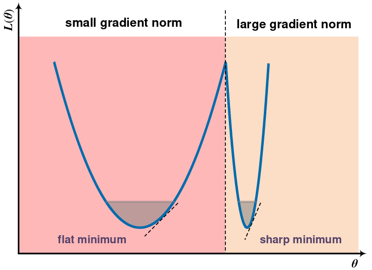
Figure 1: The gradient norm decreases as it settles into some minima (Zhao et al.).
Gradient Descent and its Variants
Original gradient descent update:
\[ \theta = \theta - \eta \nabla_{\theta}J(\theta) \]
Having a constant value for \(\eta\) means that the network will usually be unable to converge to a local minimum. As the parameters reach a minimum, the constant learning update means that it will jump around the true minimum point. This is usually remedied in part by setting up a decreasing learning rate schedule. This necessarily requires more manual guess work as to what the best annealing schedule would be.
Momentum
When the loss surface is more steep in one dimension than others, SGD will move back and forth in the directions of greatest descent while only slowly moving in the direction with a smaller decline. The figure below gives an example.
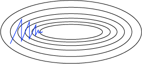
Figure 2: SGD moves slower towards covergence for non-uniform surfaces.
If the gradient had some momentum which built up over time, it would take fewer iterations to converge.
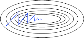
Figure 3: SGD with momentum converges in fewer iterations.
In practice, this can be implemented by adding some fraction of the previous update to the current step:
\begin{align*} \mathbf{g}_t &= \alpha \mathbf{g}_{t-1} + \eta \nabla_{\theta}J(\theta)\\ \theta &= \theta - \mathbf{g}_t \end{align*}
Nesterov Momentum
If we allow the momentum to keep increasing, the steps become greater and greater. This could lead to the parameters “rolling” out of the minimum up a steep incline. If our algorithm knew that it was coming up to an incline, it would be smarter to slow down. This is essentially what Nesterov momentum does.
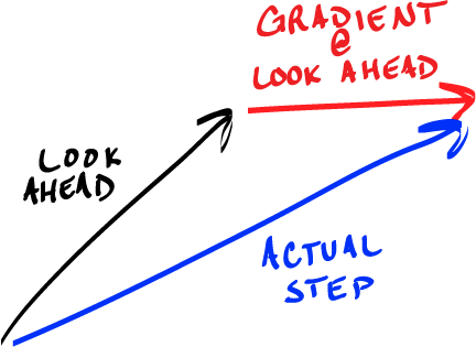
Figure 4: Nesterov momentum computes the gradient after applying momentum.
\begin{align*} \mathbf{g}_t &= \alpha \mathbf{g}_{t-1} + \eta \nabla_{\theta}J(\theta - \alpha \mathbf{g}_{t-1})\\ \theta &= \theta - \mathbf{g}_t \end{align*}
Adaptive Learning Rate Methods
The rate at which a model converges to some solution is dependent on many factors. One that we can control is the learning rate. If the learning rate is too large, the model may never converge because it jumps too far in each iteration. If the learning rate is too small, it may take much longer to converge to any solution.
It would be ideal if the optimization algorithm could adapt its learning rate to local changes in the loss landscape. In that way, the algorithm would be less dependent on the initial learning rate.
Adagrad
Adagrad adapts the learning rate to the parameters following the idea that parameters associated with salient features should be updated less frequently (Duchi, Hazan, and Singer 2011). If they occur often, updating them with a larger step would result in a solution that is more dependent on them at the expense of other features.
Adagrad uses a different learning rate for every parameter:
\[ \theta_{t+1} = \theta_t - \frac{\eta}{\sqrt{G_t + \epsilon}}g_t \]
Here, \(g_t = \frac{\partial J(\theta)}{\partial \theta}\). This provides a partial derivative for every parameter \(\theta_i\). A history of gradient changes are accumulated in a matrix \(G_t \in \mathbb{R}^{d \times d}\) which is a diagonal matrix containing the sum of squares of the gradients with respect to each \(\theta_i\) up to the current step.
In effect, the parameters with larger partial derivatives have a sharper decrease in learning rate. The downside to this method is that, as squared gradients are accumulated in \(G_t\), the sum increases causing the learning rate to eventually be too small to learn.
RMSProp
To remedy the long term issues of Adagrad, Geoffrey Hinton proposed RMSProp. There was no formal publication for this. It was discussed and taught in Coursera course on Neural Networks. Instead of accumulating gradients, RMSProp uses an exponentially weighted moving average:
\[ \mathbf{s}_t = \rho \mathbf{s} + (1 - \rho)\mathbf{g}_{t-1} \odot \mathbf{g}_t \]
A new parameter \(\rho\) controls how much of the historical gradient is used. The update is
\[ \theta_{t+1} = \theta_t - \frac{\eta}{\sqrt{\mathbf{s}_t + \epsilon}}\mathbf{g}_t. \]
Hinton proposed that \(\rho=0.9\) in the original lectures.
Adam
One of the most popular gradient descent variants in used today is Adam (Kingma and Ba 2017). Short for Adaptive Moment Estimation, Adam adapts the learning rate to each parameter. Similar to RMSProp, it stores an exponentially moving average of past squared gradients. Adam additionally stores first-order moments of the gradients.
After calculating the gradients \(g_t\) at time \(t\) the first and second moment estimates are updated as
\begin{align*} m_t &= \beta_1 \cdot m_{t-1} + (1 - \beta_1) \cdot g_t\\ v_t &= \beta_2 \cdot v_{t-1} + (1 - \beta_2) \cdot g_t^2 \end{align*}
The estimates \(m_t\) and \(v_t\) are initialized to zero leading to updated estimates that are biased to zero. The authors counteract this by computing bias-corrected estimates:
\begin{align*} \hat{m}_t &= \frac{m_t}{1 - \beta_1^t}\\ \hat{v}_t &= \frac{v_t}{1 - \beta_2^t} \end{align*}
The final update rule step is
\[ \theta_t = \theta_{t-1} - \alpha \cdot \frac{\hat{m}_t}{\sqrt{\hat{v}} + \epsilon}. \]
There are several other varients. A good overview of these can be found on Sebastian Ruder’s blog. The figures below provide some visual intuition of the behavior of common gradient descent variants. These visualizations were provided by Alec Radford.
Figure 5: Behavior of algorithms at a saddle point (Credit: Alec Radford).
Figure 6: Behavior of each algorithm on a loss surface (Credit: Alec Radford).
Additional visualizations can be found here.
Parameter Initialization
Due to the complexity of their loss landscapes, the choice of initialization can have a significant impact on the solution. This affects how quickly the model converges. Although recent work aims to smooth loss surfaces so that models are easier to train, deep learning models can be tricky to reproduce.
There is not much known about what makes the most optimal initialization strategy, but one property is that of weight symmetry. If all weights are initialized to the same value, their update will also be uniform. If two nodes are connected to the same input, there update will be uniform as well. Understanding this, a reasonable initialization strategy would be to ensure that the weights to not permit any symmetry in nodes connected to the same input.
Small weights during initialization may lead to vanishing gradients. Large weights may lead to exploding gradients as successive multiplications are applied. The parameter values should be large enough to propagate information effectively through the network.
Normalized Initialization (Xavier)
Normalized initialization chooses an initial scale of the weights of a fully connected layer based on the number input and output nodes:
\[ W_{i,j} \sim U\Bigg(-\sqrt{\frac{6}{m + n}}, \sqrt{\frac{6}{m+n}}\Bigg), \]
where \(m\) and \(n\) are the number of input and output nodes, respectively. This initialization was empirically validated by (Glorot and Bengio, n.d.) with the goal that all layers have the same activation variance and back-propagated gradient variance.
He Initialization
Xavier initialization is based on successive matrix multiplications without any non-linearities. Any deep learning model will surely break this assumption. He et al. derive another initialization strategy while considering rectified linear units (ReLU) and parametric rectified linear units (PReLU) (He et al. 2015).
Resources
-
https://spell.ml/blog/lr-schedulers-and-adaptive-optimizers-YHmwMhAAACYADm6F
References
Duchi, John, Elad Hazan, and Yoram Singer. 2011. “Adaptive Subgradient Methods for Online Learning and Stochastic Optimization.” Journal of Machine Learning Research 12 (61): 2121–59. http://jmlr.org/papers/v12/duchi11a.html.Glorot, Xavier, and Yoshua Bengio. n.d. “Understanding the Difficulty of Training Deep Feedforward Neural Networks,” 8.He, Kaiming, Xiangyu Zhang, Shaoqing Ren, and Jian Sun. 2015. “Delving Deep into Rectifiers: Surpassing Human-Level Performance on ImageNet Classification.” Arxiv:1502.01852 [Cs], February. http://arxiv.org/abs/1502.01852.Kingma, Diederik P., and Jimmy Ba. 2017. “Adam: A Method for Stochastic Optimization.” Arxiv:1412.6980 [Cs], January. http://arxiv.org/abs/1412.6980.