Patch Extraction
This post is a recreation of Misha Laskin’s Twitter post about patch extraction in numpy. I wanted to provide a version of it that can be accessed without requiring a Twitter account.
Patch extraction is a common image preprocessing technique that splits an input image into a regular grid of sub images. It is commonly used to prepare an image for input into a Vision Transformer (Dosovitskiy et al. 2021). As Misha points out in their original post, it is also used for convolutions, min and max pooling, and splicing audio and text.
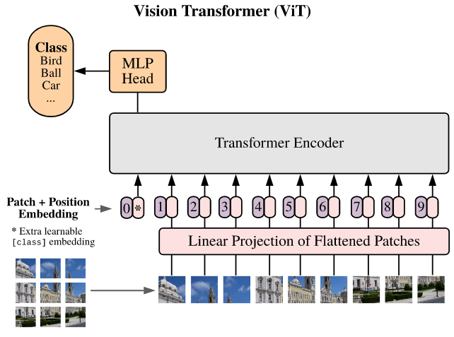
Figure 1: Patch extraction used for ViT (Dosovitskiy et al. 2021).
Native Patch Extraction
A general algorithm for patch extraction is easy enough to come up with. If the goal is to extract a grid of patches with equal size, simply loop over a grid specified by the image size and patch size.
def patch_extraction(img, size):
    H, W = img.shape
    rows, cols = H // size, W // size # rows and cols should be integers

    # initialize patches array
    patches = np.zeros((rows, cols, size, size)) # patches(0, 0) yields the first patch

    # fill in patches
    for i in range(rows):
        for j in range(cols):
            patches = img[size*i:size*(i+1), size*j:size*(j+1)]

    return patches
This naive approach essentially takes a bunch of crops of the original image. The optimization proposed by Misha takes advantage of how the array is stored in memory. The result is this: instead of extracting the patches, we can change how the array itself is accessed in memory. By default, numpy stores array elements contiguously. This is actually pretty common.
)](/ox-hugo/2024-06-06_18-12-57_screenshot.png)
Figure 2: Array elements are contiguous (Misha’s Thread)
Changing Perspective
How can we possibly change how the array is accessed? Fortunately, NumPy provides the tools do to this. A numpy array is three important properties that we will use:
shape: A list whose length is the number of dimensions of the array. Each entry of the list tells us how many elements belong to that dimension. For example, an array of shape(3, 3)has 2 dimensions, both of size 3. This would be the shape of the array seen above.strides: Represents the number of bytes needed to traverse the contiguous memory block to read the next element along a given dimension. Using the \(3 \times 3\) matrix from above, itsstridewould be(12, 4)since anintis 4 bytes, the stride is simply 4 bytes to move to the immediate next element. To traverse to the next row, you would need to move 12 bytes. This is visualized below.itemsize: The size of each element in the array.
)](/ox-hugo/2024-06-06_18-21-38_screenshot.png)
Figure 3: Visualization of strides (Misha’s Thread)
Since we already know the output shape of the patch tensor, we can specify the strides needed to get the desired patches. NumPy provides a module with a function that does this for us: stride_tricks.as_strided.
from numpy.lib import stride_tricks

# non-overlapping patches of size 8
size = 8
H, W = img.shape
shape = [H // size, W // size] + [size, size]

# (row, col, patch_row, patch_col)
strides = [size * s for s in img.strides] + list(img.strides)
# extract patches
patches = stride_tricks.as_strided(img, shape=shape, strides=strides)
The Mechanics of as_strided
How does as_strided work? Consider the example below, where we break a \(4 \times 4\) matrix into a \(2 \times 2\) array of patches, where each patch is \(2 \times 2\).
)](/ox-hugo/2024-06-06_18-29-29_screenshot.png)
Figure 4: Breaking a matrix into patches (Misha’s Thread)
We need to provide strides for the following:
- the patch in the adjacent row
- the patch in the adjacent column
- the adjacent row within a patch
- the adjacent column within a patch
Let’s start with the patch itself. Each value in the patch is a single byte (itemsize = 1). The stride needed to get to the adjacent column is 1 and the stride needed to get to the next row is 2.
Moving between patches is a bit trickier. Since each patch only has 2 columns, moving from the first to the second patch in the same column only requires moving 2 bytes. Moving from the first row of patches to the second requires 8 bytes as seen below.
)](/ox-hugo/2024-06-06_18-37-52_screenshot.png)
Figure 5: Strides required for patches (Misha’s Thread)
What about RGB?
The process given above works great for grayscale images, but what if we want to patchify a color image? Let’s take the same \(4 \times 4\) example from above, but assume it is a 3-channel image. We can create this example quickly with numpy.
# It is common to represent images as height, width, channels.
mat = np.zeros((4, 4, 3), dtype=np.uint8)
mat.strides # (12, 3, 1)
As an RGB image, each element in the grayscale version now spans 3 values. If each element is a single byte, the stride required to access the adjacent element in the next row is 12. What does this mean for our RGB version? It means we do not have to change much. The stride across the channels is built in. As long as the output shape and strides array are configured, we are in the clear. This requires two modifications.
- Each patch is now an RGB image, so
[size, size]should be changed to[size, size, 3]. - Since the original image has 3 values for
strides, only the first two should be taken when setting up the newstrideslist:strides = [size * s for s in img.strides[:2]] + list(img.strides).
)](/ox-hugo/2024-06-06_18-52-27_screenshot.png)
Figure 6: Computing strides for RGB patch extraction (Misha’s Thread)
That’s it! Happy coding.