Perceptron
Introduction
A popular example of a Logistic Regression model is the perceptron. Proposed by Frank Rosenblatt in 1962, the perceptron is defined as a generalized linear model:
\begin{equation*} f(\mathbf{w}^T\mathbf{\phi}(\mathbf{x})), \end{equation*}
where \(\phi\) is a basis function and \(f\) is a stepwise function with the form
\begin{equation*} f(a) = \begin{cases} 1, a \geq 0\\ -1, a < 0 \end{cases} \end{equation*}
To match this, the targets will take on a value of either 1 or -1.
The Perceptron Learning Algorithm
Based on the stepwise function, the parameters \(\mathbf{w}\) should lead to outputs above 0 for one class and outputs below 0 for the other. There is 0 error with a correct classification.
The original formulation does not work well with gradient based optimization methods due to the fact that the derivative of the stepwise function is 0 almost everyone. To get around this, the perceptron criterion is used:
\begin{equation*} E(\mathbf{w}) = -\sum_i \mathbf{w}^T\phi(\mathbf{x}_i)\hat{y}_i, \end{equation*}
where \(\hat{y}_i\) is the target class (either 1 or -1).
An incorrect classification will minimize \(\mathbf{w}^T\phi_i y_i\). We can consider this loss only for misclassified patterns.
Update Steps
- For each input, evaluate \(f(\mathbf{w}^T\phi(\mathbf{x}_i))\).
- For incorrect classifications
- Add \(\phi(\mathbf{x}_i)\) to \(\mathbf{w}\) estimate for class 1
- Subtract \(\phi(\mathbf{x}_i)\) from \(\mathbf{w}\) for class 2.
Does not necessarily get better each step, but guaranteed to converge.
Limitations of Single-Layer Perceptrons
Single layer perceptrons are limited to solving linearly separable patterns. As we have seen with a few datasets now, expecting our data to be linearly separable is wishful thinking. Minsky and Papert exposed this limitation in their book Perceptrons: an introduction to computational geometry.
Consider the example XOR problem. It is a binary classification problem consisting of 4 data points. It is not linearly separable as seen in the figure below.
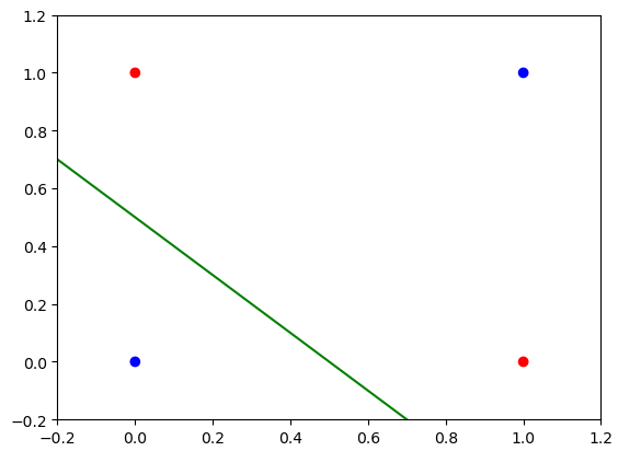
Figure 1: XOR cannot be solved with a linear classifier.
This is the result of using only a single Perceptron. What if we added another perceptron? A single perceptron computes \(\mathbf{w}^T + b\). It is important to transform the first perceptron’s output using a non-linear activation function, otherwise the output would be similar to that of a logistic regression model. The updated “network” is shown below.
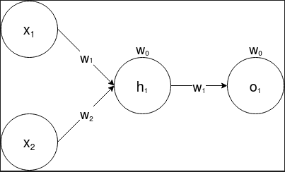
Figure 2: A 2 layer perceptron for which each layer has a single node.
The result is the same! The original input in 2D is transformed to a single dimensional output. This is then used as input to the second perceptron. The result is a linear decision boundary followed by another linear decision boundary. What if we used 2 perceptrons in the first layer? The idea is that using two linear decision boundaries in a single space would allow our model to create a more complex boundary. The updated network is shown below.
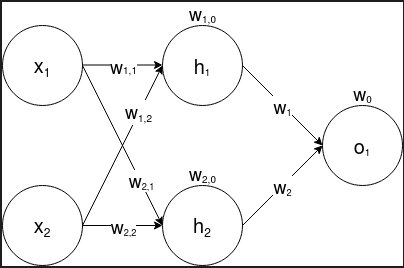
Figure 3: A 2 layer perceptron for which the first layer has 2 nodes.
This effectively solves the XOR problem! Since each node computes a linear combination of the input, we can visualize two decision boundaries with respect to the input space.
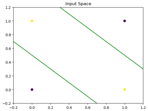
Figure 4: Visualization of input space.
Similarly, we can visualize how the data points are transformed by visualizing the space of the output layer.
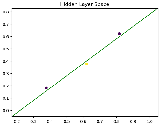
Figure 5: Output space