Principal Component Analysis
Summary
If we have some measurements of data, but do not know the underlying dynamics, PCA can resolve this by producing a change of basis such that the dynamics are reflected upon the eigenvectors.
Maximum Variance Formulation
Although there are several derivations of PCA. I really like the approach of projecting the data onto a lower dimensional space in order to maximize the variance of the projected data.
Let \(\mathbf{X}\) be a dataset of \(N\) samples, each with \(D\) features. The goal of PCA is to project this data onto an $M$-dimensional space such that \(M < D\).
Remember that the goal here is to maximize the variance of the projected data.
How do we project the data? Let’s say that we want to go from $D$-dimensional space to $M$-dimensional space where \(M = 1\). Let the vector \(\mathbf{u}\) define this 1D space. If \(\mathbf{u}\) is a unit vector, then the scalar projection of a data point \(\mathbf{x}\) onto \(\mathbf{u}\) is simply \(\mathbf{u} \cdot \mathbf{x}\).
Since we are maximizing variance, we need to subtract the mean sample from our data
\begin{equation*} \mathbf{\bar{x}} = \frac{1}{N}\sum_{n=1}^{N}\mathbf{x}_n \end{equation*}
Then, the mean of the projected data is \(\mathbf{u} \cdot \mathbf{\bar{x}}\).
With the mean of the projected data, we can calculate the variance:
\begin{equation*} \frac{1}{N}\sum_{n=1}^{N}\{\mathbf{u}^T\mathbf{x}_n - \mathbf{u}^T\mathbf{\bar{x}}\}^2 = \mathbf{u}^T\mathbf{S}\mathbf{u} \end{equation*}
where
\begin{equation*} \mathbf{S} = \frac{1}{N}\sum_{n=1}^{N}(\mathbf{x}_n - \mathbf{\bar{x}})(\mathbf{x}_n - \mathbf{\bar{x}})^T \end{equation*}
Thus, if we are maximizing the variance of the projected data, then we are maximizing \(\mathbf{u}^T\mathbf{S}\mathbf{u}\)!
So this is an optimization problem, but there is one minor issue to deal with: if \(\mathbf{u}\) is not constrained, then we scale it to infinity while maximizing the function.
Before, we stated that \(\mathbf{u}\) is a unit vector. Thus, the constraint is that \(\mathbf{u} \cdot \mathbf{u} = 1\).
After reviewing Lagrangian multipliers…
To enforce this constraint, we can use a lagrangian multiplier:
\begin{equation*} \mathcal{L}(\mathbf{u}, \lambda) = \mathbf{u}^T\mathbf{S}\mathbf{u} + \lambda(1 - \mathbf{u}^T\mathbf{u}). \end{equation*}
Let’s see what happens when we compute the stationary points (critical points) of the given Lagrangian function.
\begin{equation*} \nabla_{\mathbf{u}}\mathcal{L}(\mathbf{u}, \lambda) = \mathbf{S}\mathbf{u} - \lambda \mathbf{u} = 0 \end{equation*}
This implies that
\begin{equation*} \mathbf{S}\mathbf{u} = \lambda \mathbf{u} \end{equation*}
That particular equation means that \(\mathbf{u}\) is an eigenvector of \(\mathbf{S}\) with \(\lambda\) being the corresponding eigenvalue. Since \(\mathbf{u}\) is a unit vector, we can conveniently left-multiply both sides of that equation by \(\mathbf{u}^T\), resulting in:
\begin{equation*} \mathbf{u}^T\mathbf{S}\mathbf{u} = \lambda \end{equation*}
What does this mean?
That means that the variance is maximized when \(\mathbf{u}\) is the eigenvector corresponding to the largest eigenvalue \(\lambda\).
We can repeat this process to find the direction (eigenvector) corresponding to the second largest variance by considering eigenvectors that are orthogonal to the first one. This is where an orthonormal eigenbasis comes in handy.
Motivating Example
Consider a frictionless, massless spring that produces dynamics in a single direction.
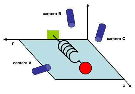
Figure 1: Toy model of spring with ball observed from 3 perspectives.
We can clearly understand that the spring will only move in a single direction. That movement reflects the underlying dynamics of this data. To understand how PCA can be useful in this situation, let’s pretend that we do not know the underlying dynamics. Instead, we observe that the data seems to go back and forth along a single axis. We observe the data over time from 3 different perspectives given by the cameras in the above figure.
From the perspective of the observer, we are recording some observations in an effort to understand which dimensions are the most salient at representing the underlying mechanics. From the above figure, we know that the most important dimension in this system is that of the labeled x-axis.
How would we figure this out if we did not already know that?
Each camera has its own coordinate system (basis). If each camera gives us a 2D location of the ball relative to that camera’s basis, then each sample in time gives us a 6D vector of locations.
Equivalently, every time sample is a vector that lies in an $m$-dimensional vector space spanned by an orthonormal basis.
Is it possible to find another basis that best expresses the data?
Mathemtically, is there some matrix \(P\) that changes our original data \(X\) into a new representation \(Y\)?
\(PX = Y\)
Noise and Redundancy
When observing real data, we will have to account for noisy measurements. Noise can come from a wide variety of sources. Being able to reduce it or filter it out is vital to understanding the underlying system.
Noise is an arbitrary measurement and means nothing without some measurement of a signal. Thus, we typically measure the amount of noise in our system using a Signal-to-Noise Ratio (SNR). This assumes we have some idea of what our signal is. This is usually given based on the nature of whatever problem we are investigating. In the toy example, we know that the spring largely moves in a single dimension. That is the signal we expect to observe.
For arguments sake, imagine we that the recordings over time from a single camera plot the following data:
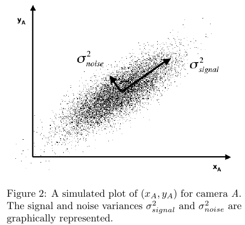
From our advantageous position of knowing the true nature of the problem, we understand there really should be no noise. However, let’s say that our camera has some noise in interpreting the precise location of the ball at any given time. In this case, our SNR is quite high, which is good! Ideally, it would be a straight line.
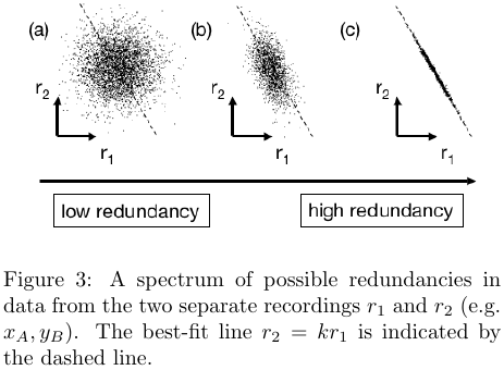
There is a second factor to consider: the fact that we are taking measurements from multiple sensors means that there may be some redundancy among the data collected from them. If we were to discover features that have high redundancy, we could be confident in concluding that they are highly correlated.
Covariance Matrix
Let \(X\) be a an \(m \times n\) matrix of \(n\) observations with \(m\) features per observation.
We can produce a covariance matrix of the features via \(S_{X} = \frac{1}{n-1}XX^{T}\).
This gives us a measurement of the correlations between all pairs of measurements.
If we want to reduce redunancy between separate measurements (those in the off-diagonal of the matrix), we would then want to diagonalize this matrix. In terms of the equation \(PX=Y\), this has the effective of finding a new covariance matrix \(S_{Y}\) that is diagonal. This means that each value in the off-diagonal of \(S_{Y}\) is 0.
PCA has a convenient assumption: the change of basis matrix \(P\) is orthonormal. Why is this convenient? PCA can then select the normalized direction in the feature space for which the variance in the data is maximized. This is called the first principal component. Because we assume \(P\) is orthonormal, the subsequent principal components must be orthogonal to the previously discovered components.
One more thing If \(P\) is not orthonormal, then we can simply scale our eigenvectors to maximize variance.