Quicksort
The lecture slides for these notes are available here.
Quicksort is a popular sorting algorithm implemented in many language libraries that has a worst-case running time of \(\Theta(n^2)\). Why would anyone choose this as the default sorting algorithm if one like mergesort has better worst-case performance? As you will see, the devil is in the details. Quicksort is often faster in practice. It also has a small memory footprint and is easy to implement.
Basic Quicksort
Quicksort follows a divide-and-conquer approach to sorting. Given an input array of \(n\) elements, it selects a pivot element and partitions the array into two sub-arrays: one with elements less than the pivot and one with elements greater than the pivot. It then recursively sorts the sub-arrays. Since the subarrays are recursively sorted, there is no need for a merge step as in mergesort.
def quicksort(arr, p, r):
    q = partition(arr, p, r)
    quicksort(arr, p, q - 1)
    quicksort(arr, q + 1, r)
This algorithm looks deceptively simple. The complexity is hidden in the partitioning step. This procedure will rearrange the elements in the array such that the pivot element is in its final position and all elements less than the pivot are to the left of it and all elements greater than the pivot are to the right of it.
Partitioning
For basic quicksort, the first or last element is chosen as the pivot. Picking it this way yields a fairly obvious recurrence of \(T(n) = T(n-1) + O(n)\), which is \(\Theta(n^2)\). As mentioned before, this algorithm is executed in-place, meaning there is no need for additional memory to store the sub-arrays. It is done through a clever use of indices.
def partition(arr, p, r):
    x = arr[r]
    i = p - 1
    for j in range(p, r):
        if arr[j] <= x:
            i += 1
            arr[i], arr[j] = arr[j], arr[i]
    arr[i + 1], arr[r] = arr[r], arr[i + 1]
    return i + 1
The indices are used to define the following loop invariant.
- Left: if \(p \leq k \leq i\), then \(A[k] \leq x\)
- Middle: if \(i + 1 \leq k \leq j - 1\), then \(A[k] > x\)
- Right: if \(k = r\), then \(A[k] = x\)
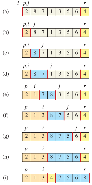
Figure 1: Operation of partition (Cormen et al. 2022).
The figure above is from CRLS which shows an example run of the partitioning algorithm. It starts with \(i, p, j\) on the left and \(r\) on the right. Since the value at \(j\) is less than the pivot, \(i\) is incremented and the values at \(i\) and \(j\) are swapped. In the next iteration, the value at \(j\) is greater than the pivot, so nothing is done. This continues until \(j\) reaches \(r\). At this point, the pivot is swapped with the value at \(i + 1\).
Example
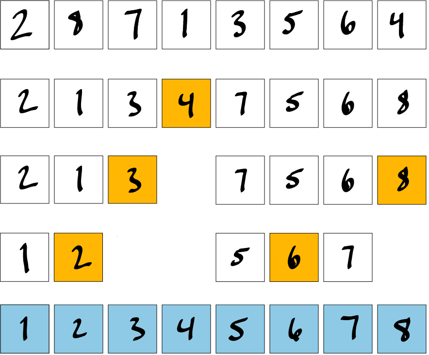
Figure 2: Example of Quicksort.
The example above starts with an unsorted array. The second row shows the array after the first call to partition. The left and right subarrays are called recursively. The first subarray in row 3 has a pivot 3 and is already partitioned. The right subarray follows the same convenience.
On row 4, the left subarray is modified by swapping the pivot of 2 with 1. The right subarray first swaps 5 and 7 before swapping 6 and 7. The final array is sorted as shown on the last row.
Performance
The performance of quicksort is dependent on the pivot. If the subarrays on either side of the pivot are balanced, the running time is asymptotically similar to mergesort. In the worst case, it will run in quadratic time.
The worst partitioning occurs when the pivot is the smallest or largest element in the array. This creates a subarray of size \(n - 1\) and another of size 0. The partitioning itself takes \(\Theta(n)\) time, yielding a recurrence of \(T(n) = T(n - 1) + \Theta(n)\). We can use the substitution method to solve this recurrence and find that the worst-case running time is \(\Theta(n^2)\). This can happen even if the input is already sorted before hand.
Cormen et al. present a recursive analysis of the running time where, at each level, the partition produces a 9-to-1 split. This is visualized in the sketch below.
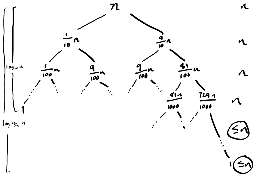
Figure 3: Recursion tree for quicksort.
The subtree for the \(\frac{1}{10}\) split eventually bottoms out after being called \(\log_{10} n\) times. Until this happens, the cost of each level of the tree is \(n\). After the left-tree bottoms out, the right tree continues with an upper bound of \(\leq n\). The right tree completes after \(\log_{10/9} n = \Theta(\lg n)\) levels. Since each level of the tree cost no more than \(n\), the total cost is \(\Theta(n \lg n)\).
Best Case
In the best-case, the pivot is the median of the array and two balanced subarrays are created: one of size \(n/2\) and another of size \(\lfloor (n-1)/2 \rfloor\). The recurrence is \(T(n) = 2T(n/2) + \Theta(n)\), which is \(\Theta(n \log n)\).
Using the substitution method, we can show the best-case running time. We start with the fact that the partitioning produces two subproblems with a total size of \(n-1\). This gives the following recurrence:
\[ T(n) = \min_{0 \leq q \leq n-1} \{T(q) + T(n - q - 1)\} + \Theta(n). \]
The minimum function accounts for the minimum time taken to sort any partition of the array, where \(q\) represents the pivot element’s position.
Our hypothesis will be that
\[ T(n) \geq cn \lg n = \Omega(n \lg n). \]
Plugging in our hypothesis, we get
\begin{align*} T(n) &\geq \min_{0 \leq q \leq n-1} \{cq \lg q + c(n - q - 1) \lg (n - q - 1)\} + \Theta(n) \\ & c \min_{0 \leq q \leq n-1} \{q \lg q + (n - q - 1) \lg (n - q - 1)\} + \Theta(n). \end{align*}
If we take the derivative of the function inside the minimum with respect to \(q\), we get
\[ \frac{d}{dq} \{q \lg q + (n - q - 1) \lg (n - q - 1)\} = c\{\frac{q}{q} + \lg q - \lg (n - q - 1) - \frac{(n - q - 1)}{(n - q - 1)}\}. \]
Setting this equal to zero and solving for \(q\) yields
\[ q = \frac{n - 1}{2}. \]
We can then plug this value of \(q\) into the original function to get
\begin{align*} T(n) &\geq c \frac{n - 1}{2} \lg \frac{n - 1}{2} + c \frac{n - 1}{2} \lg \frac{n - 1}{2} + \Theta(n) \\ &= cn \lg (n - 1) + c (n - 1) + \Theta(n) \\ &= cn \lg (n - 1) + \Theta(n) \\ &\geq cn \lg n \\ &= \Omega(n \lg n). \end{align*}
Average Case
As it turns out, the average-case running time is \(\Theta(n \log n)\) (Cormen et al. 2022). Quicksort is highly dependent on the relative ordering of the input. Consider the case of a randomly ordered array. The cost of partitioning the original input is \(O(n)\). Let’s say that the pivot was the last element, yielding a split of 0 and \(n - 1\). Now, let’s say we get lucky on the next iteration and get a balanced split. Even if the rest of the algorithm splits between the median and the last element, the upper bound on the running time is \(\Theta(n \log n)\). It is highly unlikely that the split will be unbalanced on every iteration given a random initial ordering.
We can make this a tad more formal by defining a lucky \(L(n) = 2U(n/2) + \Theta(n)\) and an unlucky split \(U(n) = L(n-1) + \Theta(n)\). We can solve for \(L(n)\) by plugging in the definition of \(U(n)\).
\begin{align*} L(n) &= 2U(n/2) + \Theta(n) \\ &= 2(L(n/2 - 1) + \Theta(n/2)) + \Theta(n) \\ &= 2L(n/2 - 1) + \Theta(n) \\ &= \Theta(n \log n) \end{align*}
Randomized Quicksort
The intuition of the crude analysis above is that we would have to be extremely unlucky to get a quadratic running time if the input is randomly ordered. Randomized quicksort builds on this intuition by selecting a random pivot on each iteration. This is done by swapping the pivot with a random element before partitioning.
import random

def randomized_partition(arr, p, r):
    i = random.randint(p, r)
    arr[i], arr[r] = arr[r], arr[i]
    return partition(arr, p, r)

def randomized_quicksort(arr, p, r):
    if p < r:
        q = randomized_partition(arr, p, r)
        randomized_quicksort(arr, p, q - 1)
        randomized_quicksort(arr, q + 1, r)
Analysis
The lightweight analysis above reasoned that, as long as each split puts a constant amount of elements to one side of the split, then the running time is \(\Theta(n \log n)\).
We can understand this analysis simply by asking the right questions. First, our primary question: What is the running time of Quicksort dependent on? The biggest bottleneck is the partitioning function. At most, we get really unlucky and the first pivot is picked every time. This means it is called \(n\) times yielding \(O(n)\). The variable part of this is figuring out how many element comparisons are made. The running time is then \(O(n + X)\).
The Expected Value of \(X\)
The number of comparisons can be expressed as
\[ X = \sum_{i=1}^{n-1} \sum_{j=i+1}^{n} X_{ij}, \]
where \(X_{ij}\) is the indicator random variable that is 1 if \(A[i]\) and \(A[j]\) are compared and 0 otherwise. This works with our worst case analysis. If we always get a split of 0 and \(n - 1\), then the indicator random variable is 1 for every comparison, yielding \(O(n^2)\). Taking the expectation of both sides:
\begin{align*} E[X] &= E\left[\sum_{i=1}^{n-1} \sum_{j=i+1}^{n} X_{ij}\right] \\ &= \sum_{i=1}^{n-1} \sum_{j=i+1}^{n} E[X_{ij}] \\ &= \sum_{i=1}^{n-1} \sum_{j=i+1}^{n} P(X_{ij} = 1). \end{align*}
What is \(P(X_{ij} = 1)\)? Let \(z_i, \dots, z_j\) be the indices of elements in a sorted version of the array. Under this assumption, \(z_i\) is compared to \(z_j\) only if \(z_i\) or \(z_j\) is the first pivot chosen from the subarray \(A[i \dots j]\). In a set of distinct elements, the probability of picking any pivot from the array from \(i\) to \(j\) is \(\frac{1}{j - i + 1}\). This means that the probability of comparing \(z_i\) and \(z_j\) is \(\frac{2}{j - i + 1}\). We can now finish the calculation.
\begin{align*} E[X] &= \sum_{i=1}^{n-1} \sum_{j=i+1}^{n} \frac{2}{j - i + 1} \\ &= \sum_{i=1}^{n-1} \sum_{k=1}^{n-i} \frac{2}{k + 1} \\ &< \sum_{i=1}^{n-1} \sum_{k=1}^{n-i} \frac{2}{k} \\ &= \sum_{i=1}^{n-1} O(\log n) \\ &= O(n \log n). \end{align*}
Paranoid Quicksort
Repeat the following until the partitioning until the left or right subarray is less than or equal to \(\frac{3}{4}\) of the original array.
- Choose a random pivot.
- Partition the array.
- Verify that the left and right subarrays are less than or equal to \(\frac{3}{4}\) of the original array.
- If not, repeat the partitioning.
- Recursively sort the subarrays.
Analysis
Most of the analysis of Paranoid Quicksort follows that of randomized quicksort. The focus is on the expected number of calls times partition is called until no side of the split is greater than \(\frac{3}{4}\) of the input.
Consider a sorted array of \(n\) distinct elements. The first and last \(\frac{n}{4}\) elements would produce a bad split. That means there are \(n/2\) values that provide a good split, implying that \(p(\text{good split}) = \frac{1}{2}\). Knowing the probability of this event means we can calculated the expected number of times we should call partition before getting a good split, which is 2.
Continuing on with this analysis, we need to state the recurrence:
\[ T(n) \leq 2cn + T(\lfloor 3n/4) \rfloor) + T(\lceil n/4 \rceil) + O(1) \]
The addition of \(2cn\) is not enough to change our analysis from above. Thus, the expected running time of Quicksort is \(O(n \log n)\).