RANdom SAmple Consensus
Introduction
Unless our data is perfect, we will not be able to find parameters that fit the data in the presence of outliers. Consider fitting the data in the figure below using a least squares method.
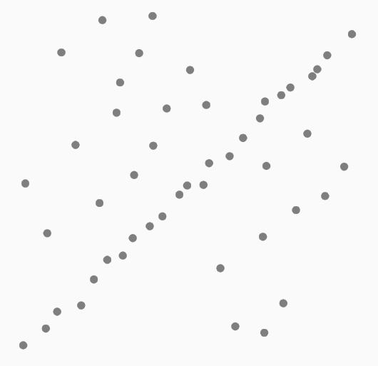
Figure 1: Points sample along a line with many outliers around it. Source: Wikipedia
If we were to fit a naive least squares model, the outliers would surely produce parameters for a line that does not fit the most amount of data possible.
Consider the figures below. In the first one, a least squares model is fit to points generated from a line. With the addition of just a single outlier, the model no longer fits the line.
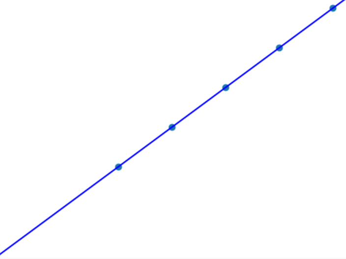
Figure 2: Least squares can easily fit a line with great accuracy.
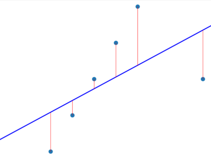
Figure 3: A single outlier leads to a bad fit for linear regression.
Ideally, we want a model that is robust to outliers. That is, the model should be fit such that it matches the largest number of samples, or inliers. One such approach to this problem is RANdom SAmple Consensus (RANSAC).
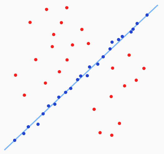
Figure 4: RANSAC fit to most inliers while ignoring the outliers. Source: Wikipedia
The general process is as follows:
- Randomly select source samples and their matching targets.
- Fit a model to the data such that transforming the input by the model parameters yields a close approximation to the targets.
- Measure the error of how well ALL data fits and select the number of inliers with error less than \(t\).
- If the error is lower than the previous best error, fit a new model to these inliers.
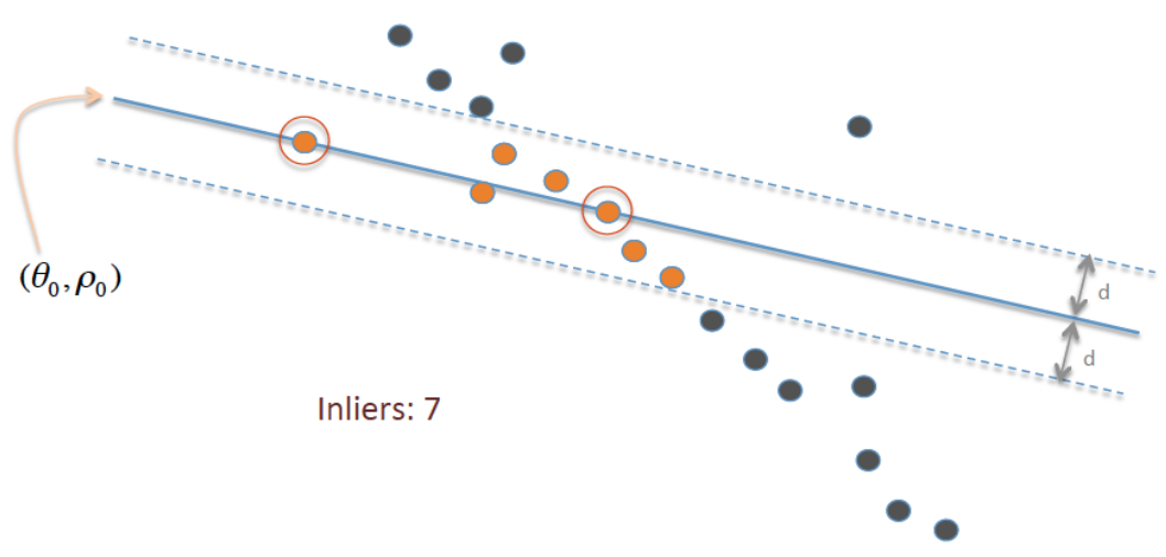
Figure 5: RANSAC fitting random samples and counting the number of inliers. Source: Wikipedia
The algorithm can be found on the Wikipedia page.
Finding the Best Fit Model
When it comes to finding the parameters of a transformation matrix that converts points in one image to another, how do we solve for that matrix? We are looking for some \(A\) such that
\begin{equation*} A\mathbf{x} = \mathbf{\hat{x}}. \end{equation*}
In a perfect world, \(\mathbf{\hat{x}}\) will match the target point \(\mathbf{y}\). In other words,
\(\|\mathbf{\hat{x}} - \mathbf{y}\|_{2} = 0\).
For an affine transformation, we would have some transformation matrix
\begin{equation*} A = \begin{bmatrix} a_{11} & a_{12} & a_{13}\\ a_{21} & a_{22} & a_{23} \end{bmatrix}. \end{equation*}
Then we compute each component of \(A\mathbf{x}\) as
\begin{align*} \hat{x}_1 &= a_{11} * x_1 + a_{12} * x_2 + a_{13} * 1\\ \hat{x}_2 &= a_{21} * x_1 + a_{22} * x_2 + a_{23} * 1\\ \end{align*}
We can fit this using a least squares approach by the following construction.
\begin{equation*} \begin{bmatrix} x_1^{(1)} & x_2^{(1)} & 1 & 0 & 0 & 0\\ 0 & 0 & 0 & x_1^{(1)} & x_2^{(1)} & 1\\ && \vdots\\ x_1^{(n)} & x_2^{(n)} & 1 & 0 & 0 & 0\\ 0 & 0 & 0 & x_1^{(n)} & x_2^{(n)} & 1\\ \end{bmatrix} \begin{bmatrix} a_{11}\\ a_{12}\\ a_{13}\\ a_{21}\\ a_{22}\\ a_{23}\\ \end{bmatrix}= \begin{bmatrix} \hat{x}_1^{(1)}\\ \hat{x}_2^{(1)}\\ \vdots\\ \hat{x}_1^{(n)}\\ \hat{x}_2^{(n)}\\ \end{bmatrix} \end{equation*}
We can solve this analytically! Recall the normal equations:
\[ A^T A \mathbf{x} = A^T \mathbf{b}. \]
Let’s test this on a couple of images…
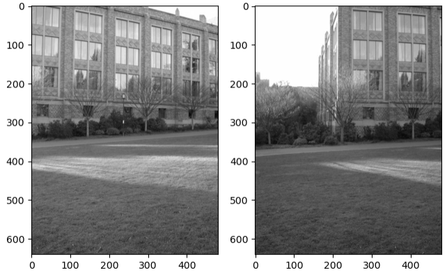
Figure 6: Two images taken with matching features shared between them.
First, we use some feature detector such as SIFT to find keypoints in each image. Then, we can take a brute force approach to determine which keypoints match between them.
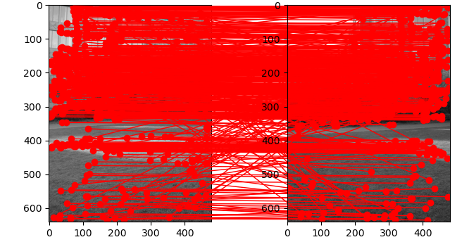
Figure 7: We’ve got a lot of potential matches here.
After running RANSAC, we end up with a model that fits the following inlier points.
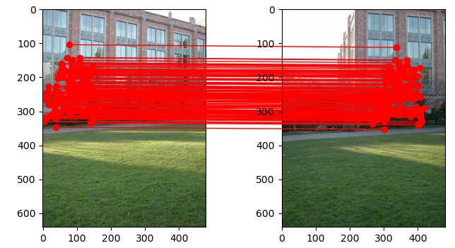
Figure 8: Many of the outliers were removed and we are left with the following matches.
We can use the found transformation matrix to warp our source image to fit our destination image as seen below.
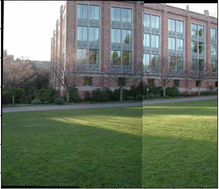
Figure 9: Images stitched together… not perfect!
Finding a better transformation
The transformation matrix was an affine transformation matrix. What we really want is a projective transformation! We can extend our approach to finding an affine matrix from earlier by remembering that projective transformations are completed following a perspective divide (usually denoted by \(w\)).
Instead of a constant 1 in the third position of the affine vector, we have a value \(w\):
\begin{equation*} \begin{bmatrix} a_{11} & a_{12} & a_{13}\\ a_{21} & a_{22} & a_{23}\\ a_{31} & a_{32} & a_{33}\\ \end{bmatrix} \begin{bmatrix} x\\ y\\ w \end{bmatrix}= \begin{bmatrix} \hat{x}\\ \hat{y}\\ \hat{w} \end{bmatrix}. \end{equation*}
Dividing by \(\hat{w}\) completes the perspective projection:
\begin{equation*} \begin{bmatrix} \frac{\hat{x}}{\hat{w}}\\ \frac{\hat{y}}{\hat{w}}\\ 1 \end{bmatrix}. \end{equation*}
Again, we can write out the individual equation for each component as
\begin{align*} \hat{x} &= (a_{11} * x + a_{12} * y + a_{13} * w) \div (a_{31} * x + a_{32} * y + a_{33} * w)\\ \hat{y} &= (a_{21} * x + a_{22} * y + a_{23} * w) \div (a_{31} * x + a_{32} * y + a_{33} * w)\\ \end{align*}
We may assume that \(w = 1\) for the original points (before transformation). Additionally, \(a_{33}\) is typically set to 1 when constructing a transformation matrix. These are safe enough assumptions to make considering that we will make many attempts at finding the best fitting parameters.
Solving for \(\hat{x}\) and \(\hat{y}\) in terms of a linear combination of elements yields
\begin{align*} \hat{x} &= a_{11} * x + a_{12} * y + a_{13} - \hat{x} * a_{31} * x - \hat{x} * a_{32} * y\\ \hat{y} &= a_{21} * x + a_{22} * y + a_{23} - \hat{y} * a_{31} * x - \hat{y} * a_{32} * y\\ \end{align*}
We can fit this using a least squares approach by the following construction.
\begin{equation*} \begin{bmatrix} x_1^{(1)} & x_2^{(1)} & 1 & 0 & 0 & 0 & -x_1^{(1)}\hat{x}_1^{(1)} & -x_2^{(1)}\hat{x}_1^{(1)}\\ 0 & 0 & 0 & x_1^{(1)} & x_2^{(1)} & 1 & -x_1^{(1)}\hat{x}_2^{(1)} & -x_2^{(1)}\hat{x}_2^{(1)}\\ && \vdots\\ x_1^{(n)} & x_2^{(n)} & 1 & 0 & 0 & 0 & -x_1^{(n)}\hat{x}_1^{(n)} & -x_2^{(n)}\hat{x}_1^{(n)}\\ 0 & 0 & 0 & x_1^{(n)} & x_2^{(n)} & 1 & -x_1^{(n)}\hat{x}_2^{(n)} & -x_2^{(n)}\hat{x}_2^{(n)} \end{bmatrix} \begin{bmatrix} a_{11}\\ a_{12}\\ a_{13}\\ a_{21}\\ a_{22}\\ a_{23}\\ a_{31}\\ a_{32} \end{bmatrix}= \begin{bmatrix} \hat{x}_1^{(1)}\\ \hat{x}_2^{(1)}\\ \vdots\\ \hat{x}_1^{(n)}\\ \hat{x}_2^{(n)} \end{bmatrix}. \end{equation*}
We can use the normal equations as before to solve for this system.
The figure below shows the final result of image stitching using a perspective projection instead of an affine matrix.
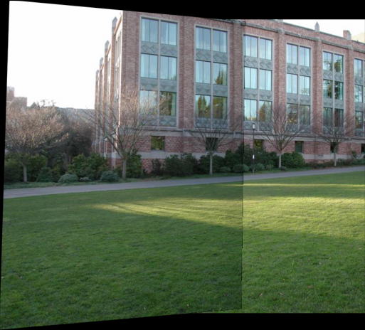
Figure 10: Stitching using a perspective projection.