Recurrent Neural Networks
Introduction
Neural networks are an effective tool for regression and classification tasks, but they do not consider the dependencies of information over time. Many tasks have implicit information that is dependent on input that may have already been processed or may not be seen until the future.
Recurrent Neural Networks (RNN) consider the historical context of time-series data. Bi-directional Recurrent Neural Networks (BRNN) consider both historical and future context. This is necessary for tasks like language tanslation.
Parameter sharing across different parts of the model is key for sequence models. Different instances of a particular feature may appear at different time steps.
“I see Naomi there.” and “Naomi is right there” both convey that Naomi is present, but we would not require the model to have separate parameters just because the word position is different between the two.
Recurrent connections provide a memory of sorts. This enables important contextual information to be “remembered” throughout time. These models are not without their limitations. When trained with gradient descent, the gradient information passed throughout multiple time steps can become insignificant. There are several ways to address the vanishing gradient problem which are explored in alternative models such as Long Short-Term Memory and Transformers.
Definition
The definition of RNNs start with that of Neural Networks. One layer of an RNN has some number of hidden units that transforms the input into an intermediate representation. In addition to transforming the input, another set of parameters is used to transform the hidden context over time. The difference is that the hidden layer is shared over time, as seen in the equation below.
\[ \mathbf{h}^{(t)} = f(\mathbf{h}^{(t-1)}, \mathbf{x}^{(t)}; \mathbf{\theta}) \]
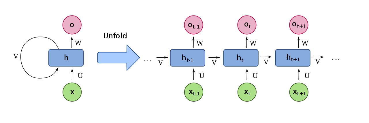
Figure 1: Computation graph of an RNN (By fdeloche - Own work, CC BY-SA 4.0, https://commons.wikimedia.org/w/index.php?curid=60109157)
In the computation graph above, a recurrent network has three weight matrices associated with its forward pass. An input weight matrix \(U \in \mathbb{R}^{H \times D}\) processes the features for each frame of the input sequence. The hidden layer has a weight matrix \(V \in \mathbb{R}^{H \times H}\), where \(H\) is the number of hidden nodes. The output layer will have a weight matrix \(W \in \mathbb{R}^{O \times H}\).
Forwards Pass
To understand the computation graph of an RNN, consider an input of length \(T\) with \(D\) features. That is, each input sample is a sequence of features. This could be represented as encoded video data, text data, or any other sequence signals. To compute the output of a hidden layer \(\mathbf{h}\) at time \(t\), take a linear combination of all input feature \(x_i^t\) at time \(t\) in addition to the output of the previous hidden layer and then add the linear combination of output activations for each node in the hidden layer:
\[ a_h^t = \sum_{d=1}^D w_{dh} x_d^t + \sum_{h’=1}^H w_{h’h} b_{h’}^{t-1}, \]
where \(b_h^t = \theta_h(a_h^t)\) and we assume the bias term is concatenated with the weights.
Weights in the hidden layer are crucial for RNNs to adapt to contextual features based on their occurrence relative to time. For example, a character-based language model based on a traditioinal network would produce similar output for consecutive letters that are the same. In an RNN, the hidden weights would produce a different output for each consecutive character even if it were the same.
The hidden layer outputs are used in both the subsequent computations through time as well as the output node for each instance \(t\). The inputs to the output node are computed from the hidden node at the same time as the output to the hidden activation:
\[ a_k^t = \sum_{h=1}^H w_{hk}b_h^t. \]
Backwards Pass
The gradients of a recurrent network are computed using backpropagation, similar to neural networks. Since the forward pass is over \(t\) time step, the backward pass must consider them as well. This variant of backpropagation for recurrent models is calling backpropagation through time (BPTT).
Like a feed forward network, the output is dependent on the activation of the hidden layer. For a recurrent model, its dependence is through the output of the hidden layer as well as the pass to the next hidden time step.
\[ \frac{\partial \mathcal{L}}{\partial a_h^t} = \frac{\partial \mathcal{L}}{\partial b_h^t} \frac{\partial b_h^t}{\partial a_h^t} \]
\[ \frac{\partial \mathcal{L}}{\partial b_h^t} = \sum_{k=1}^K \frac{\partial \mathcal{L}}{\partial a_k^t} \frac{\partial a_k^t}{\partial b_h^t} + \sum_{h’=1}^H \frac{\partial \mathcal{L}}{\partial a_{h’}^{t+1}} \frac{\partial a_{h’}^{t+1}}{\partial a_{h}^t} \]
The derivatives with respect to the weights are given as
\[ \frac{\partial \mathcal{L}}{\partial w_{ij}} = \sum_{t=1}^T \frac{\partial \mathcal{L}}{\partial a_j^t} \frac{\partial a_j^t}{\partial w_{ij}}. \]
Bidirectional Recurrent Neural Networks
Standard RNNs work for many problems with sequential input. Training such a model would consider the full input through time \(T\), but inference may only be able to consider the data up to time \(t < T\). There are sequential tasks which could leverage from both past and future context, such as language translation. For this case, BRNNs were proposed <&schusterBidirectionalRecurrentNeural1997>.

Figure 2: Diagram of BRNN from Graves et al.
References
- The Unreasonable Effectiveness of RNNs by Andrej Karpathy
- <&gravesSupervisedSequenceLabelling2012>
- Understanding LSTM Networks by Christopher Colah