Sampling and Aliasing
Resizing
- Aliasing arises through resampling an image
- How to resize - algorithm
- How to resolve aliasing
Resizing an image, whether increase or decreasing the size, is a common image operation. In Linear Algebra, scaling is one of the transformations usually discussed, along with rotation and skew. Scaling is performed by creating a transformation matrix
\begin{equation*} M = \begin{bmatrix} s & 0\\ 0 & s \end{bmatrix}, \end{equation*}
where \(s\) is the scaling factor. This matrix can then be used to transform the location of each point via matrix multiplication.
Is is that simple for digital images? Can we simply transform each pixel location of the image using \(M\)? There are a couple of steps missing when it comes to scaling digital images. First, \(M\) simply creates a mapping between the location in the original image and the corresponding output location in the scaled image. If we were to implement this in code, we would need to take the pixel’s value from the original image.
A Simple example
Take a \(2 \times 2\) image whose pixel values are all the same color.
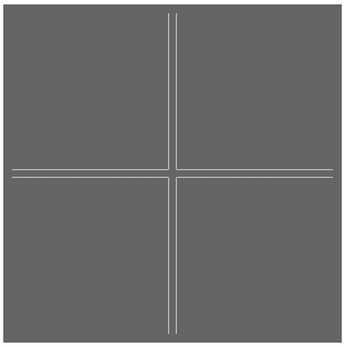
Figure 1: 2 by 2 image whose values are the same.
If we transform each pixel location of the image and copy that pixel’s value to the mapped location in the larger image, we would get something as seen in the figure below.
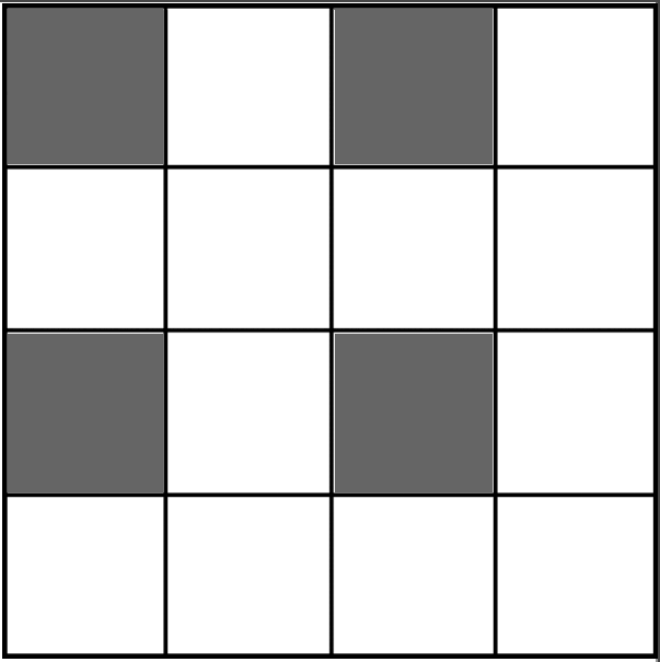
Figure 2: The resulting scaled image.
This image is exactly what we would expect. The resulting image is two times as large as the first. What pixel values should the new ones take on? This is a question of sampling.
Sampling
Given \(s = 2\), the scaling matrix maps the original pixel locations to their new values:
- \((0, 0) \mapsto (0, 0)\)
- \((0, 1) \mapsto (0, 2)\)
- \((1,0) \mapsto (2, 0)\)
- \((1,1) \mapsto (2, 2)\)
What values should be given to the unmapped values of the new image? There are several sampling strategies used in practice. Two of the most common approaches are nearest neighbor and bilinear sampling. Let’s start with the nearest neighbor approach.
Nearest Neighbor
First, we let the pixel location in an image be the center of that pixel, as depicted below.
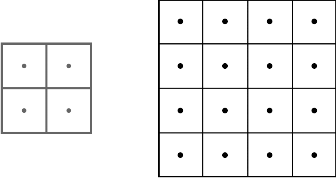
Figure 3: A 2-by-2 image with pixel locations depicted as dots in the center.
To establish a map between the pixel locations in the scaled image and that of the original image, we shrink the grid on the larger image and superimpose it over the smaller image.
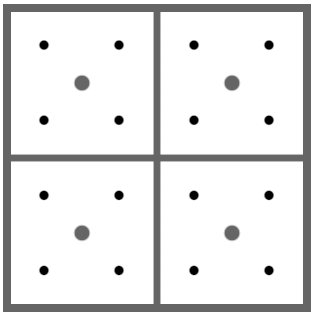
Figure 4: Pixel grid of larger image superimposed on original image.
With nearest neighbor interpolation, the pixel value in the resized image corresponds to that of the nearest pixel in the original image. In the above figure, we can see that pixels \((0, 0), (0, 1), (1, 0), \text{ and } (1, 1)\) in the resized image are closest to pixel \((0, 0)\) in the original image. Thus, they will take on that pixel’s value.
Let’s compare both of these approaches on a real image. The first figure below shows the original image \((16 \times 16\)). The following figure shows the image resized to \((32 \times 32)\) with no interpolation and nearest neighbor interpolation, respectively.
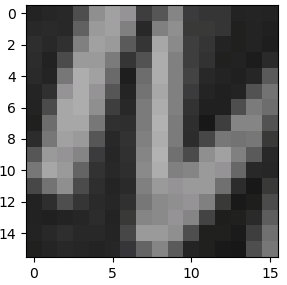
Figure 5: Original image.
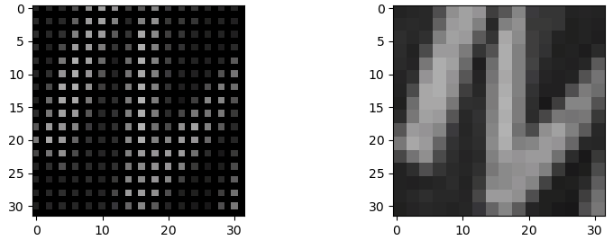
Figure 6: Image resized with no interpolation (left) and nearest neighbor (right).
Bilinear Interpolation
Bilinear interpolation is a slightly more sophisticated way of sampling which takes into account all neighboring pixels in the original image. The value of the pixel in the sampled image is a linear combination of the values of the neighbors of the corresponding pixel it is mapped to.
Consider a \(3 \times 3\) image upsampled to a \(8 \times 8\) image. The figure below shows the original image with the coordinates of the upsampled image superimposed on it.
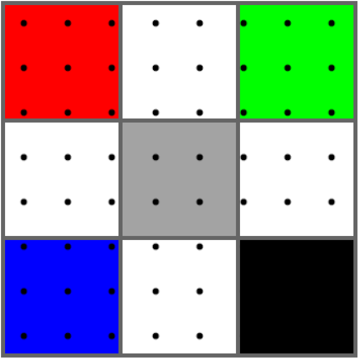
Figure 7: 3-by-3 grid with 8-by-8 coordinates overlaid.
How do we determine the coordinate map between the original and upscaled image? Solve a linear system.
Note the extreme values of the image. That is, the smallest and largest coordinates. Since we stated previously that \((0, 0)\) refers to the coordinate in the middle of the pixel, the top-left of the image boundary for any image is \((-0.5, -0.5)\). The bottom-right corner for the smaller image is \((2.5, 2.5)\). The bottom-right corner for the resized image is \((7.5, 7.5)\). The equation that maps the top-left coordinates between the images is given by
\[ -\frac{1}{2} = -\frac{1}{2}a + b. \]
The equation that maps the bottom-right coordinates between the images is given by
\[ \frac{5}{2} = \frac{15}{2}a + b. \]
Thus, we have 2 equations 2 unknowns. Solving this yields \(a = \frac{3}{8}\) and \(b = -\frac{5}{16}\).
With the mapping solved, let’s compute the color value for pixel \((3, 3)\) in the upsampled image. Here, \((3, 3) \mapsto (\frac{13}{16}, \frac{13}{16})\) in the original image. Our problem for this particular pixel is reduced to the following figure.
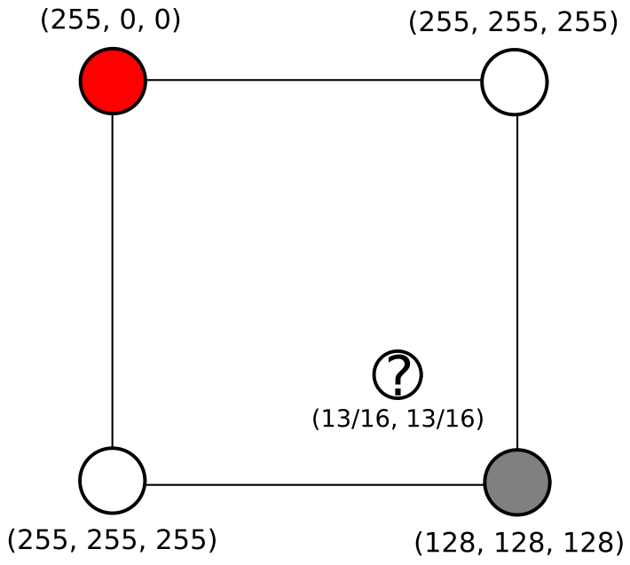
Figure 8: Determining the pixel value for the mapped pixel using bilinear interpolation.
We first interpolate between two pairs of pixels in the original image. That is, we find \(p_1\) and \(p_2\) in the following figure.
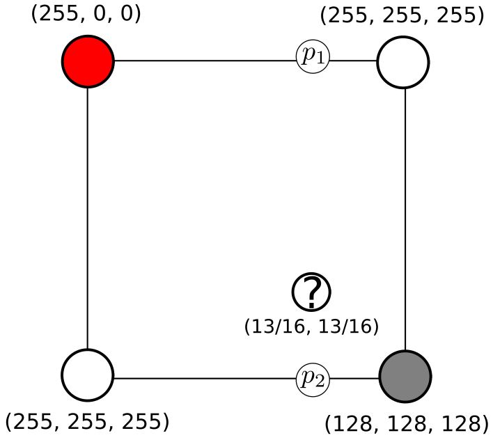
Figure 9: Step 1: Interpolate the pixel values between two pixels for (p_1) and (p_2).
Here, \(p_2 = \frac{3}{16}(255, 255, 255) + \frac{13}{16}(128, 128, 128) \approx (152, 152, 152)\) and \(p_1 = \frac{3}{16}(255, 0, 0) + \frac{13}{16}(255, 255, 255) \approx (255, 207, 207)\). Note that the contribution of the pixel depends on the weight on the other side the intermediate value \(p_i\). For example, if you think of \(p_1\) as a slider from the red pixel to the white pixel. The value to the left of the slider reflects the contribution of the pixel to the right, and vice versa.
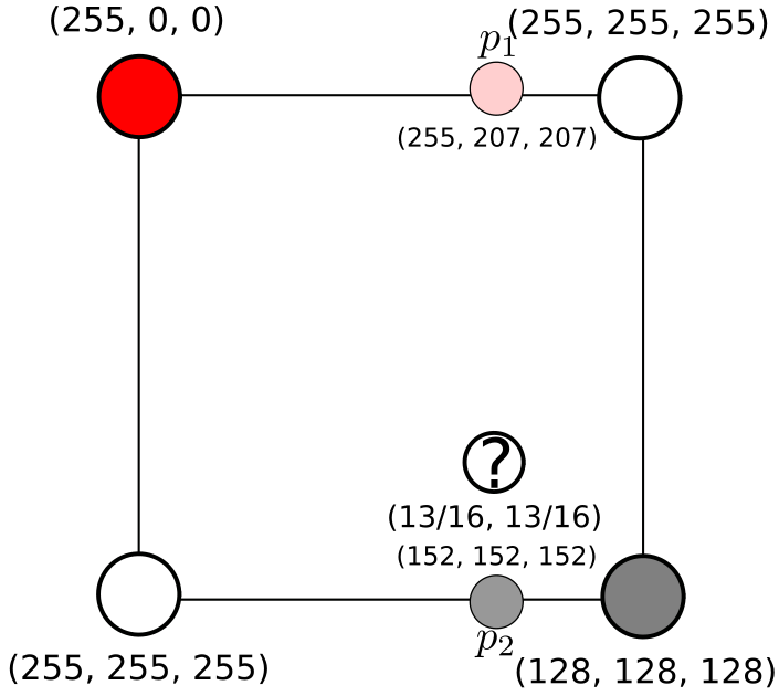
Figure 10: Computed values of (p_1) and (p_2).
Finally, the value of the new pixel is a linear combination of \(p_1\) and \(p_2\). That is \(p = \frac{13}{16}(152, 152, 152) + \frac{3}{16}(255, 207, 207) \approx (171, 162, 162)\).
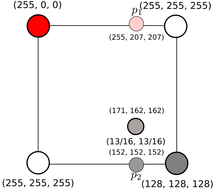
Figure 11: The final pixel value computed from (p_1) and (p_2).
The following figure compares the original image with both types of interpolation discussed in this section.
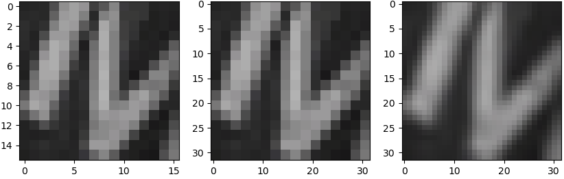
Figure 12: Original image (left), upscaled 2x with NN interpolation (middle), upscaled with bilinear interpolation (right).
Aliasing
Nearest neighbor interpolation often leads to images with aliasing. In general, aliasing occurs when two signals are sampled at such a frequency that they become indistinguishable from each other. Usually, images are smoothed prior to upsampling or downsampling in an effort to alleviate the effects of aliasing. The figure below shows a downsampled image using nearest neighbor interpolation.
Figure 13: Image downsampled by 4x. Notice the “jaggies”, especially along straight lines.
By blurring the image and using bilinear interpolation, the same image looks much smoother when downsized.
Figure 14: Image downsampled by 4x using bilinear interpolation.