Scale Invariant Feature Transforms
The goal is to detect features that are robust to varying conditions like scale, rotation, and translation. SIFT focuses first on detection of scale-space extrema. A robust feature is one that is invariant to scale change. If this feature appears consistently as the scale space is changed, it will ultimately be selected.
Scale-Space Extrema
Detecting features that are robust to changes in scale is arguably the most important property of this work. As discussed in Image Features, features across multiple scales can be detected by using the Laplacian of Gaussian. In Lowe’s paper, extrema are detected more efficiently by approximating this function.
Scale space in this context is defined as \(L(x, y, \sigma) = G(x, y, \sigma) * I(x, y)\), where \(G\) is a Gaussian kernel. Extrema in scale-space indicate locations with in the image with a large gradient magnitude. In other words, edges, corners, and other texture rich features.
Difference of Gaussians
This same technique for detecting interesting points in a scale-invariant way can be approximated by taking the Difference of Gaussians. Consider the figure below.
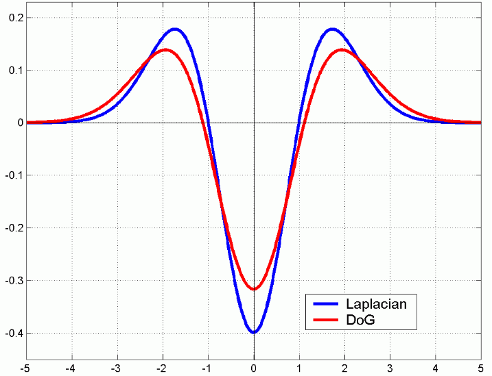
Figure 1: Comparison of DoG and Laplacian. Credit: Fei-Fei Li.
By taking the difference of images smoothed by a Gaussian with different values of \(\sigma\), the resulting pixel values correspond to areas with high gradient norms in the less blurry version.
Let \(I_{\sigma_1}\) be the image blurred with a smaller value of \(\sigma\) and \(I_{\sigma_2}\) be the image blurred with a larger value. Then \(D(I_{\sigma_1}, I_{\sigma_2}) = I_{\sigma_2} - I_{\sigma_1}\). If a region in \(I_{\sigma_1}\) is locally flat, it will also be in flat in \(I_{\sigma_2}\). The difference will be relatively small for that region. If there are abrupt changes in a local region within \(I_{\sigma_1}\), they will be smoothed in \(I_{\sigma_2}\). Therefore, the difference \(D(I_{\sigma_1}, I_{\sigma_2})\) will be higher for that region.
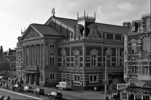
Figure 2: The Royal Concertgebouw in Amsterdam.
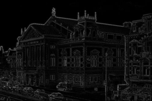
Figure 3: Difference of Gaussian between the original image blurred with (sigma = 0.5) and (sigma=1.5).
Theoretical Justification for DoG
Based on previous work by Lindeberg, it was shown that scale-normalization of the Laplacian of Gaussian with a factor of $\sigma^2$ is required for scale invariance. Further, the difference of Gaussian across a constant factor of $\sigma$ is approximately equal to the scale-normalized Laplacian of Gaussian:
$$ G(x, y, k\sigma) - G(x, y, \sigma) \approx (k - 1)\sigma^2 \nabla^2 G. $$
When building SIFT features, the extremum are selected by comparing 3 DoG images. These are selected by evaluating each pixel to 26 of its neighbors in the current scale space and neighboring DoG spaces as visualized below.
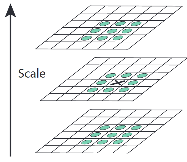
Figure 4: Finding extrema of pixel (i, j) in a neighborhood of 26 values (Lowe 2004).
To build the DoG pyramid, the authors propose that images are separated by a constant factor \(k\) in scale space. Each octave of scale space is divided such that the scale-space doubles every \(s\) samples.
Starting with \(\sigma = 0.5\), if we choose \(s=3\) then the fourth sample will be at \(\sigma = 1\), the seventh at \(\sigma=2\), and so on. To make sure the DoG images cover the full range of an octave, \(s + 3\) images need to be created per octave.
Why \(s + 3\)?
Each octave should evaluate local extrema for \(s\) scales. To evaluate this for scale \(\sigma_s\), we need DoG images for scales \(\sigma_{s-1}\), \(\sigma_{s}\), and \(\sigma_{s+1}\). This would require 4 Gaussians images to compute. The figure below represents the stack for \(s=2\).
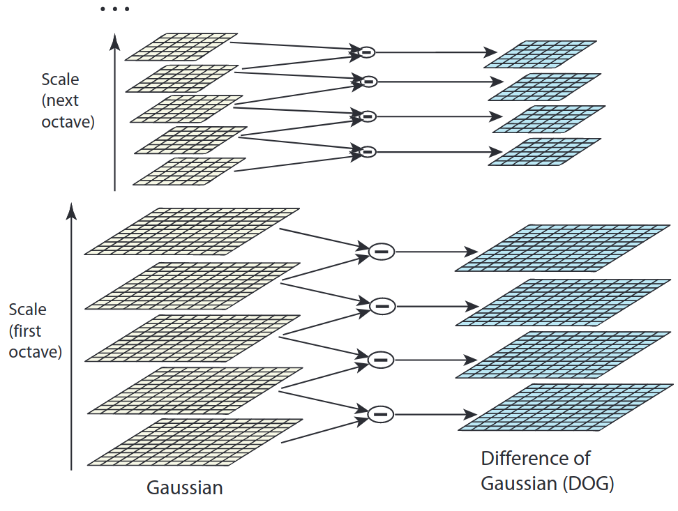
Figure 5: DOG figure (Lowe 2004).
Example With $S=3$
If $s=3$, then $k=2^{\frac{1}{3}} \approx 1.26$.
Starting with $\sigma_0 = 1$, the subsequent values are $[\sigma_0, \sigma_1, \sigma_2, \sigma_3, \sigma_4, \sigma_5] = [1, k, k^2, k^3, k^4, k^5]$.
Note that $\sigma$ is doubled at $k^3$, corresponding to the image that is 2 below the top of the stack (as stated by Lowe).
If we only want a doubling of $\sigma$, why are we computing $k^4 \approx 2.51$ and $k^5 \approx 3.17$?
The extrema detection requires 3 DoG images. Therefore, the detection at $D(x, y, \sigma^3)$ (doubling) also requires the DoG above and below it. To generate those 3 images we need $\sigma_2, \sigma_3, \sigma_4,$ and $\sigma_5$.
How is the value of \(s\) determined?
In the paper, the authors perform a repeatability test to determine if the keypoints would be localized even with random augmentations. The process is as follows:
- Randomly augment an input image with noise, color jitter, scale, rotation, etc.
- Compute keypoints using using the extrema detection.
- Compare detected keypoints with known keypoints from original samples.
The authors found that using \(s = 3\) provided the highest percentage of repeatability in their experiments.
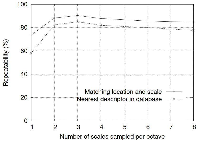
Figure 6: Measuring repeatability of keypoint detections versus # of scales sampled per octave (Lowe 2004).
Keypoint Localization
Given the candidate keypoints selected by picking out local extrema, they pool of responses can further be refined by removing points that are sensitive to noise or located along an edge. They borrow the same approach used in the Harris corner detector to select more robust interest points in corners.
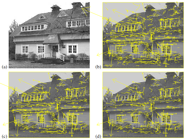
Figure 7: Refinement of candidate keypoints by filtering those sensitive to noise (c) and those representing ambiguity along edges (d) (Lowe 2004).
Orientation Assignment
Given a keypoint, an orientation histogram is generated. The authors use 36 bins to cover a 360 degree range for orientations. Similar to Histogram of Oriented Gradients, the orientations are weighted by their gradient magnitudes (Dalal and Triggs 2005). Additionally, a Gaussian-weighted circular patch is applied, centered on the keypoint, to further weight the responses. This means that points farther away from the center contribute less to the overall feature vector.
In order to make the keypoint rotation invariant, the dominant orientation is determined. If there are orientations that are within 80% of the highest orientation peak, multiple keypoints will be created using those orientations as well.
Orientations in this window are rotated by the dominant gradient so that all directions are with respect to the dominant orientation. This is a more efficient alternative to rotating the entire image by that orientation.
Descriptor Formation
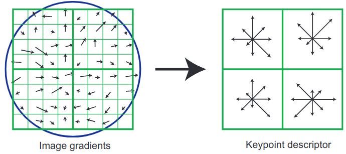
Figure 8: Keypoint descriptor generation (Lowe 2004).
In the paper, the authors generate keypoints using a \(16 \times 16\) window from which \(4 \times 4\) descriptors are generated following the descriptions above. Through experimentation, each \(4 \times 4\) descriptor uses 8 orientations, resulting in a feature vector \(\mathbf{x} \in \mathbb{R}^{128}\).
Different levels of contrast will product edges with higher gradient magnitudes. To account for this, the final feature vector is normalized using the \(L2\) hysteresis approach used in Harris corner detection.