Segmentation via Clustering
Introduction
The goal of segmentation is fairly broad: group visual elements together. For any given task, the question is how are elements grouped? At the smallest level of an image, pixels can be grouped by color, intensity, or spatial proximity. Without a model of higher level objects, the pixel-based approach will break down at a large enough scale.
Segmentation by thresholding works in cases where the boundaries between features are clearly defined. However, thresholding is not very robust to complex images with noise. Consider a simple image and its intensity histogram as noise is added.
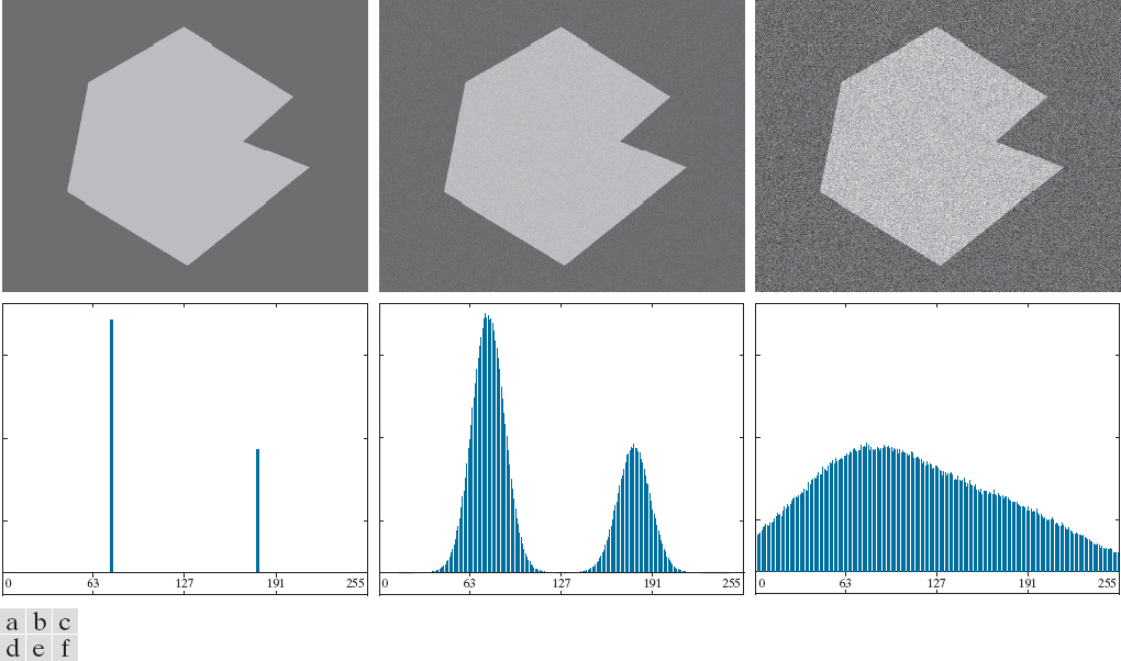
Figure 1: From left to right, a noiseless image with increasing amounts of Gaussian noise added. Source: Pearson Education, Inc.
Even with some noise added, as seen in the middle image, thresholding is still relatively straightforward. Once enough noise is added, thresholding via pixel intensities will not work. A more sophisticated approach is needed in this case.
Clustering is a fairly intuitive way to think about segmentation. Instead of a fine-grained representation of an image as a collection of pixels, it is represented as groups or clusters that share some common features. The general process of clustering is simple. The image is represented as a collection of feature vectors (intensity, pixel color, etc.). Feature vectors are assigned to a single cluster. These clusters represent some segment of the image.
When it comes to clustering methods, there are two main approaches: agglomerative and divisive. Simply, one is a bottom-up approach. The other is a top-down approach. After briefly introductin agglomerative clustering, we will explore specific implementations of segmentation using k-means clustering as well as segmentation using superpixels <&achantaSLICSuperpixelsCompared2012>.
Agglomerative Clustering
Agglomerative clustering methods start by assuming every element is a separate cluster. Elements are formed based on some local similarities. As these methods iterate, the number of clusters decreases. Deciding which elements to merge depends on inter-cluster distance. The exact choice of distance is dependent on the task. Some examples include:
- Single-link clustering: The distance between the closest elements.
- Complete-link clustering: The maximum distance between an element of the first cluster and one of the second.
- Group average clustering: Average distance of elements in a cluster.
How many clusters are or should be in a single image?
This is a difficult question to answer for many reasons. The answer will be largely dependent on the task at hand. It is a problem of learning the underlying generative process of the visual elements in the image. By defining the specific goal of segmentation (segment by color, shape, etc.), we are introducing a prior about the underlying generative processes which formed the image.
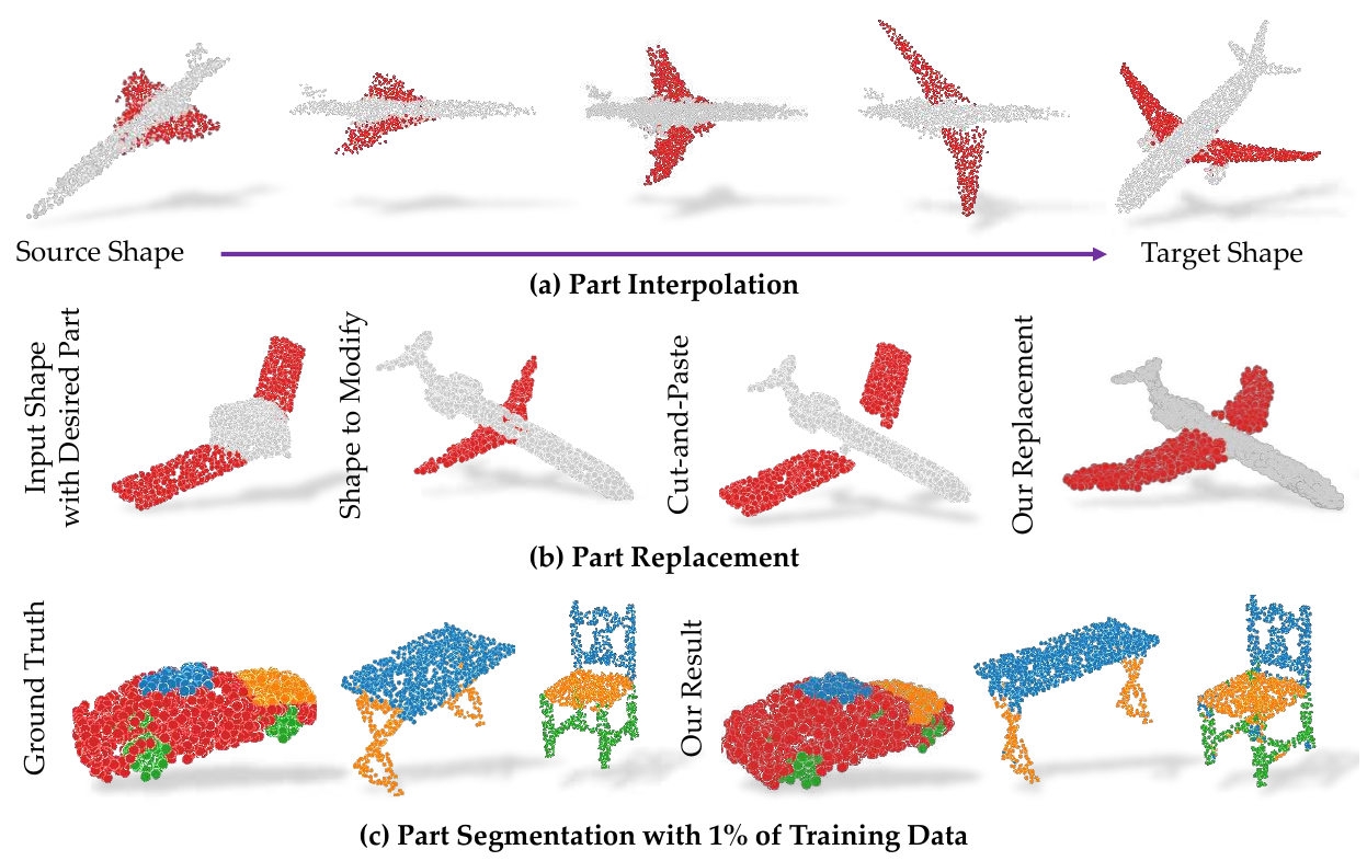
Figure 2: 3D-PointCapsNet learns point segmentations on only 1% of the training data (Zhao et al.).
There are approaches which attempt to segment objects in semi-supervised settings. As seen in Figure 1, Zhao et al. propose a part segmentation model for 3D objects which only utilizes 1-5% of the training part labels <&zhao3DPointCapsule2019>.
For example, if we divised an algorithm that would segment an image by color values, it might be able to segment the hand wearing a solid color glove relatively easily. If we wanted to segment the hand into its individual joints, we would have to introduce a visual prior such as asking the subject to wear a multicolored glove. We could also add prior information about the hand shape and joint configuration into the model itself.
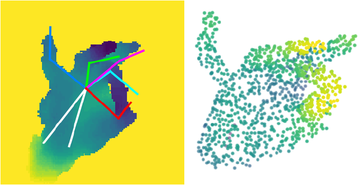
Figure 3: An image-based joint regression model predicts joint locations (left) along with a point cloud generated from the joint estimates (right).
In the figure above, the kinematic hand model could be used to segment the hand by assigning points in the point cloud to the nearest joint as estimated by the model.
One way to visualize the cluster relationships is a dendrogram. Initially, each element is its own cluster. As the process evolves and clusters are merged based on some similarity, the hierarchy is updated to show how the connections are formed.
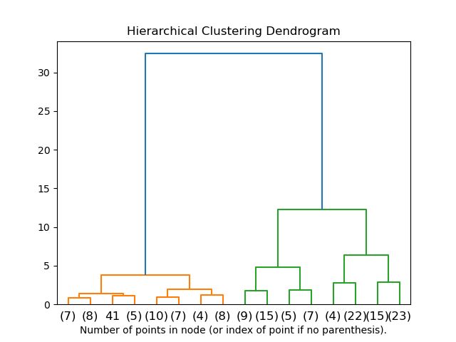
Figure 4: Example output from scikit-image.
K-Means Clustering
- K-Means Variant KNN Demo
- https://scikit-learn.org/stable/auto_examples/cluster/plot_color_quantization.html#sphx-glr-auto-examples-cluster-plot-color-quantization-py
K-Means clustering is a popular machine learning method used in both supervised and unsupervised settings. It works by iteratively updating a set of centroids or means until some stopping criteria is achieved.
To use this with image segmentation, we start by treating our image features as vectors. In the RGB case, each pixel is a vector of 3 values. It starts out by initializing \(k\) clusters randomly with means \(\mathbf{m}_i\). The next step is to compute the distance between the clusters and each point in the image. Points are assigned to the cluster that is closest.
\[ \text{arg}\min_{C} \sum_{i=1}^k \sum_{\mathbf{z}\in C_i}\|\mathbf{z} - \mathbf{m}_i\|^2, \]
where \(C = \{C_1, \dots, C_k\}\) is the cluster set.
K-Means uses Expectation Maximization to update its parameters. That is, it first computes the expected values given its current cluster centers before updating the cluster centers based on the new assignments. The standard algorithm is as follows:
- Initialize clusters - Randomly select \(k\) points as cluster centers \(\mathbf{m}_i\).
- Assign samples to clusters - Assign each sample to the closest cluster center based on some distance metric.
- Update the means - Compute a new value for the cluster centers based on the assignments in the previous step. \[ \mathbf{m}_i = \frac{1}{|C_i|}\sum_{\mathbf{z} \in C_i}\mathbf{z}, \quad i = 1, \dots, k \]
- Test for convergence - Compute the distances between the means at time \(t\) and time \(t - 1\) as \(E\). Stop if the difference is less than some threshold: \(E \leq T\).
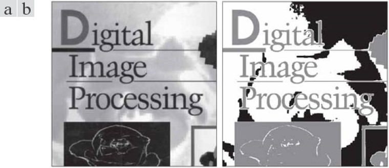
Figure 5: Image segmented using k-means with k=3. Source: Pearson Education, Inc.
Simple Linear Iterative Clustering (SLIC)
Simple Linear Iterative Clustering (SLIC) is widely used algorithm based on K-Means clustering for image segmentation <&achantaSLICSuperpixelsCompared2012>.
As discussed in the original paper, the authors state that SLIC h as two main advantages over traditional K-Means:
- The search space for assigning points is reduced, leading to an increase in performance.
- By weighting the distance measure, color and spatial proximity are both considered when forming clusters.
The algorithm itself is simple to understand and implement, as seen below.
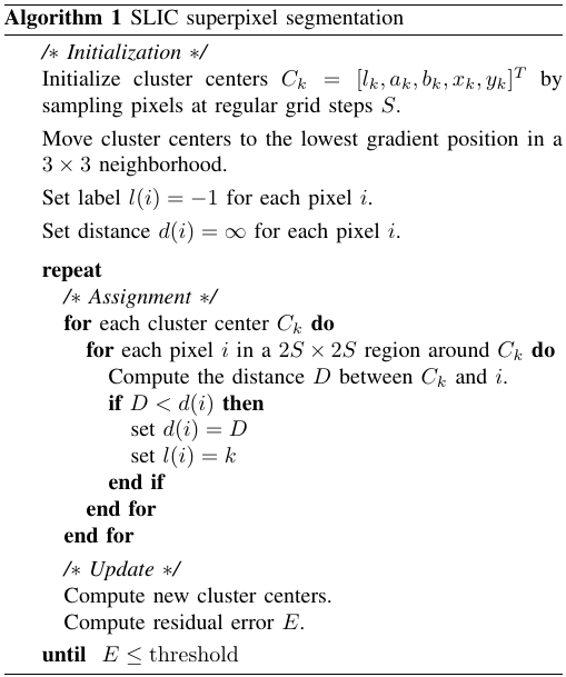
Figure 6: SLIC Algorithm (Achanta et al.)
Initialization
To keep the search space smaller, the individual search regions are spaced \(S = \sqrt{N/k}\) pixels apart, where \(N\) is the number of pixels and \(k\) is the number of cluster centers.
The image itself is represented in CIELAB color space. This color space was chosen because it is perceputally uniform. That is, it is useful for detecting small differences in color.
Each of the \(k\) pixel clusters is then defined as a superpixel consisting of the CIELAB color and position:
\[ C_i = [l_i\ a_i\ b_i\ x_i\ y_i]^T. \]
For stability, the seed locations are moved to the lowest gradient position in a \(3 \times 3\) neighborhood. If the superpixels are building locally distinct regions, it is better to avoid placing them on an edge (boundary) pixel.
Search Space and Distance
The search space for a cluster center is a region \(2S \times 2S\) around the cluster. Each pixel in this region is compared to the cluster center \(C_k\) using a distance measure \(D\).
The distance measure should consider both the spatial and color distances:
\begin{align*} d_c &= \sqrt{(l_j - l_i)^2 + (a_j - a_i)^2 + (b_j - b_i)^2}\\ d_s &= \sqrt{(x_j - x_i)^2 + (y_j - y_i)^2}\\ D’ &= \sqrt{\Big(\frac{d_c}{N_c}\Big)^2 + \Big(\frac{d_s}{N_s}\Big)^2} \end{align*}
The individual distances should be normalized by their respective maximums since the range of CIELAB values is different from the variable maximum of \(N_s\), which is based on the image size. Here, \(N_s\) corresponds to the sampling size \(\sqrt{N/k}\).
The authors found that normalizing this way was inconsistent since the color distances vary greatly from cluster to cluster. They turn this normalization into a hyperparameter constant \(m\) so that the user can control the importance between spatial and color proximity.
\[ D = \sqrt{d_c^2 + \Big(\frac{d_s}{S}\Big)^2 m^2} \]
A smaller \(m\) results in superpixels that adhere more to image boundaries, where a larger value promotes compact superpixels.
Results
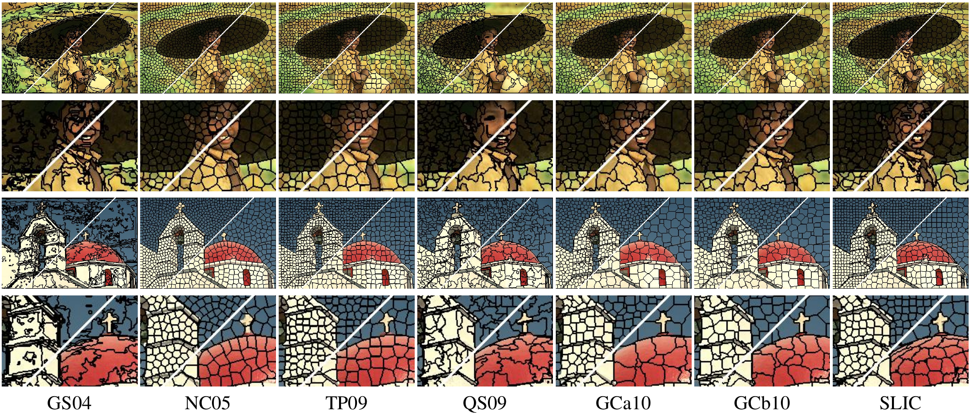
Figure 7: Comparison of SLIC against other superpixel methods (Achanta et al.)
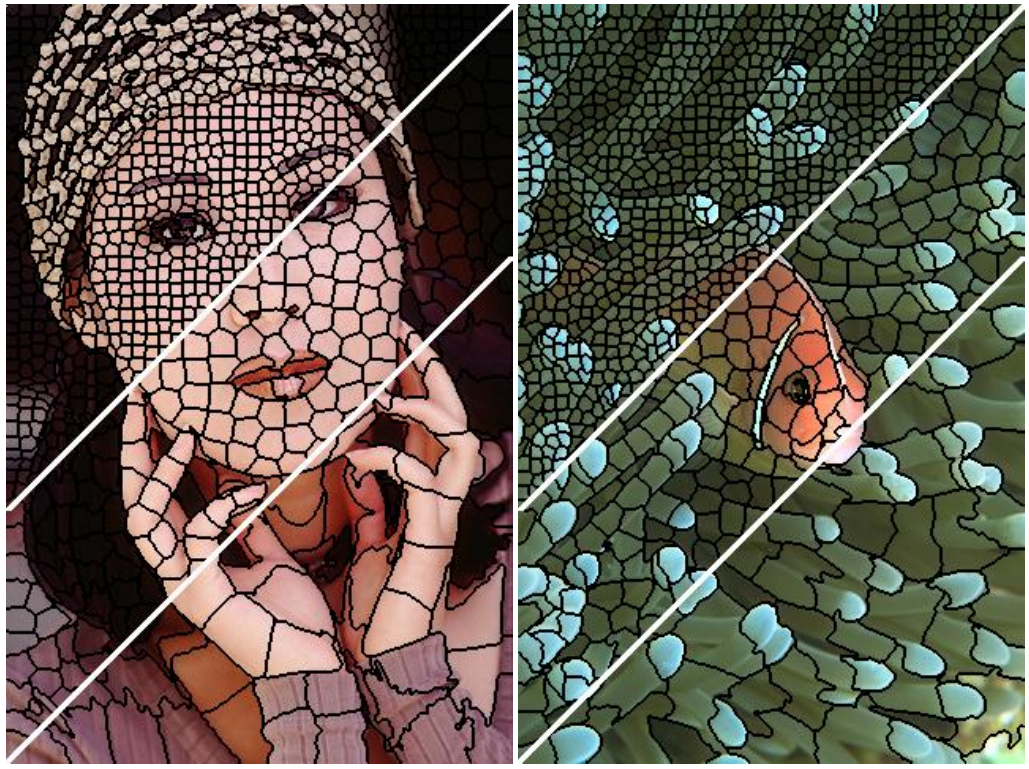
Figure 8: Images segmented using a varying number of clusters (Achanta et al.)
Superpixels in Recent Work
Superpixels are useful for reducing the dimensionality of the feature space. Their applications include tracking, segmentation, and object detection. Methods that extract superpixels do not work out of the box with deep learning methods due to their non-differentiable formulation. Deep learning methods rely on gradient descent to optimize their parameters. This requires that the functions used in a deep network be differentiable.
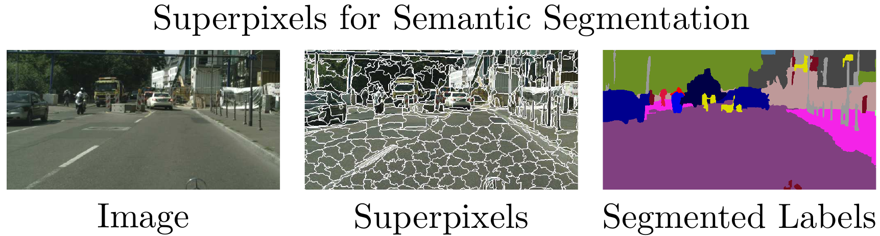
Figure 9: Superpixels optimized for semantic segmentation (Jampani et al.)
Superpixel Sampling Networks, proposed by Jampani et al., introduce the first attempt at integrating superpixel extraction methods with deep learning models <&jampaniSuperpixelSamplingNetworks2018>. In this work, they adapt SLIC as a differentiable layer in a deep network which result in superpixels that are fine-tuned for specific tasks.
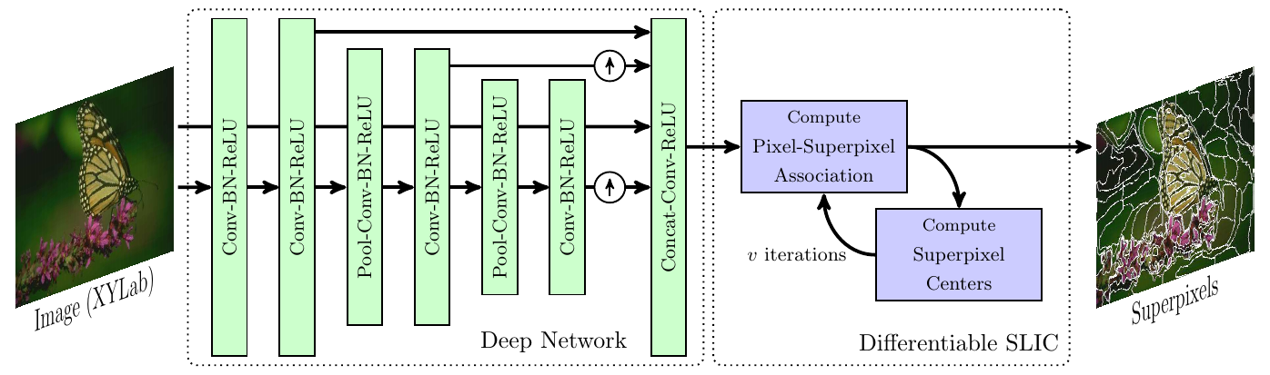
Figure 10: Model diagram for SSN (Jampani et al.)
The train their model on a semantic segmentation task which fine tunes the learned superpixels such that they adhere more closely to segmentation boundaries.
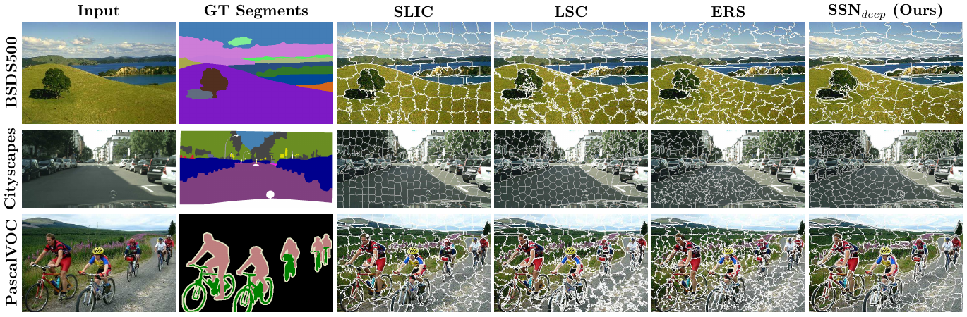
Figure 11: Results on semantic segmentation (Jampani et al.)
In a more recent work, Yang et al. propose a deep network that directly produces the superpixels as opposed to using a soft K-Means layer <&yangSuperpixelSegmentationFully2020>.
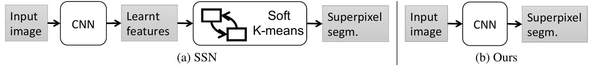
Figure 12: Model comparison between Jampani et al. and Yang et al. (Yang et al.)
Similar to SSN, they experiment on the Berkeley Image Segmentation Dataset. Their results are competitive with other deep learning-based approaches. The authors note that their method generalizes better in segmentation tasks by being robust to fine details and noise. Additionally, their model runs at 50 fps using 4 NVIDIA Titan Xp GPUs.
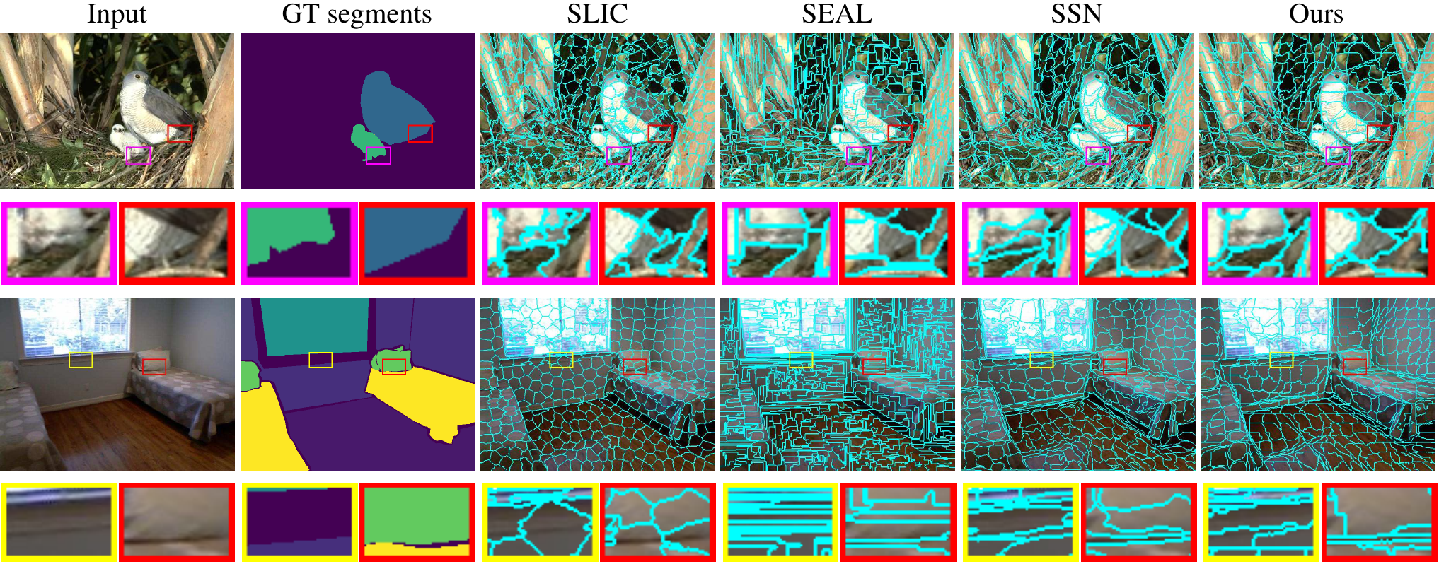
Figure 13: Comparison of results on competing methods (Yang et al.)
#print_bibliography: t