Sequential Minimal Optimization
Introduction
Sequential Minimal Optimization (SMO) is an algorithm to solve the SVM Quadratic Programming (QP) problem efficiently (Platt 1998). Developed by John Platt at Microsoft Research, SMO deals with the constraints of the SVM objective by breaking it down into a smaller optimization problem at each step.
The two key components of SMO are
- an analytic method to solving for two Lagrange multipliers at a time
- and a heuristic for choosing which multipliers to optimize.
The original objective is to maximize the margin between the nearest positive and negative examples. For the linear case, if the output is given as
\[ u = \mathbf{w}^T \mathbf{x} - b, \]
where \(\mathbf{w}\) is the normal vector to the hyperplane separating the classes, then the margin is given as
\[ m = \frac{1}{\|w\|_2}. \]
Maximizing this margin yielded the primal optimization problem
\begin{align*} \min_{\mathbf{w},b} \frac{1}{2} \|\mathbf{w}\|^2\\ \textrm{s.t.} \quad & y_i(\mathbf{w}^T \mathbf{x} - b) \geq 1, \forall i\\ \end{align*}
The dual form of the objective function for a Support Vector Machine is
\[ \min_{\vec\alpha} \Psi(\vec{\alpha}) = \min_{\vec{\alpha}} \frac{1}{2}\sum_{i=1}^N \sum_{j=1}^N y_i y_j K(\mathbf{x}_i, \mathbf{x}_j)\alpha_i\alpha_j - \sum_{i=1}^N \alpha_i \]
with inequality constraints
\[ \alpha_i \geq 0, \forall i, \]
and a linear equality constraint
\[ \sum_{i=1}^N y_i \alpha_i = 0. \]
For a linear SVM, the output is dependent on a weight vector \(\mathbf{w}\) and threshold \(b\):
\[ \mathbf{w} = \sum_{i=1}^N y_i \alpha_i \mathbf{x}_i, \quad b = \mathbf{w}^T \mathbf{x}_k - y_k. \]
The threshold is also dependent on the weight vector? The weight vector \(\mathbf{w}\) is computed using the training data. The threshold is only dependent on non-zero support vectors, \(\alpha_k > 0\).
Overlapping Distributions
Slack variables were introduced to allow misclassifications at the cost of a linear penalty. This is useful for datasets that are not linearly separable. In practice, this is accomplished with a slight modification of the original objective function:
\begin{align*} \min_{\mathbf{w},b} \frac{1}{2} \|\mathbf{w}\|^2 + C \sum_{i=1}^N \xi_i\\ \textrm{s.t.} \quad & y_i(\mathbf{w}^T \mathbf{x} - b) \geq 1 - \xi_i, \forall i\\ \end{align*}
The convenience of this formulation is that the parameters \(\xi_i\) do not appear in the dual formulation at all. The only added constraint is
\[ 0 \leq \alpha_i \leq C, \forall i. \]
This is referred to as the box constraint for reasons we shall see shortly.
Box Constraints
The smallest optimization step that SMO solves is that of two variables. Given the constraints above, the solution lies on a diagonal line \(\sum_{i=1}^N y_i \alpha_i = 0\) bounded within a box \(0 \leq \alpha_i \leq C, \forall i\).
Isolating for two samples with alphas \(\alpha_1\) and \(\alpha_2\), the constraint \(\sum_{i=1}^n y_i \alpha_i = 0\) suggests that
\[ y_1 \alpha_1 + y_2 \alpha_2 = w. \]
We first consider the case when \(y_1 \neq y_2\). Let \(y_1 = 1\) and \(y_2 = -1\), then \(a_1 - a_2 = w\). As \(\alpha_1\) increases, \(\alpha_2\) must also increase to satisfy the constraint.
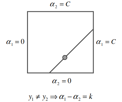
Figure 1: Equality constraint for case 1 (Platt 1998).
The other case is when \(y_1 = y_2\), then \(\alpha_1 + \alpha_2 = w\). As \(\alpha_1\) is increased, \(\alpha_2\) is decreased to satisfy the constraint.
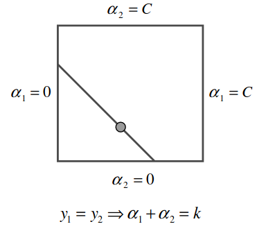
Figure 2: Box constraint for samples of the same class (Platt 1998).
Updating the Lagrangians
SMO solves for only two Lagrange multipliers at a time. Solving for only 1 at a time would be impossible under the constraint \(\sum_{i=1}^N y_i \alpha_i = 0\). The first step is to compute \(\alpha_2\) and constrain it between the ends of the diagonal line segment from the box constraints.
If \(y_1 \neq y_2\), then the following bounds are applied to \(\alpha_2\):
\begin{equation*} L = \max(0, \alpha_2 - \alpha_1), \quad H = \min(C, C + \alpha_2 - \alpha_1) \end{equation*}
otherwise, the bounds are computed as:
\begin{equation*} L = \max(0, \alpha_2 + \alpha_1 - C), \quad H = \min(C, \alpha_2 + \alpha_1) \end{equation*}
Updating the actual parameter is done following the update rule of gradient descent:
\[ \alpha_2^{\text{new}} = \alpha_2 + \frac{y_2(E_1 - E_2)}{\eta}. \]
How do we arrive at this update rule?
Second Derivative of the Objective Function
Here, \(\eta\) represents the step size and direction. It is computed from the second derivative of the objective function along the diagonal line. To see that this is the case, consider the original objective function
\begin{align*} \min_{\mathbf{\alpha}} \quad & \frac{1}{2} \sum_{i=1}^N \sum_{j=1}^N y_i y_j K(\mathbf{x}_i, \mathbf{x}_j) \mathbf{\alpha}_1 \mathbf{\alpha}_2 - \sum_{i=1}^N \alpha_i\\ \textrm{s.t.} \quad & 0 \leq \alpha_i \leq C, \forall i\\ & \sum_{i=1}^N y_i \alpha_i = 0\\ \end{align*}
Since we are optimizing with respect to only 2 Lagrangian multipliers at a time, we can write the Lagrangian function as
\[ \frac{1}{2} y_1^2 K_{11} \alpha_1^2 + \frac{1}{2} y_2^2 K_{22} \alpha_2^2 + y_1 \alpha_1 \sum_{j=3}^N y_j \alpha_j K_{1j} + y_2 \alpha_2 \sum_{j=3}^N y_j \alpha_j K_{2j} - \alpha_1 - \alpha_2 + \sum_{j=3}^N \alpha_j \]
We are only optimizing with respect to \(\alpha_1\) and \(\alpha_2\), the next step is to extract those terms from the sum. This is simplified further by noting that \(\sum_{j=3}^N y_j \alpha_j K_{ij}\) looks very similar to the output of an SVM:
\[ u = \sum_{j=1}^N y_j \alpha_j K(\mathbf{x}_j, \mathbf{x}) - b. \]
This allows us to introduce a variable \(v_i\) based on \(u_i\), the output of an SVM given sample \(\mathbf{x}_i\):
\[ v_i = \sum_{j=3}^N y_j \alpha_j K_{ij} = u_i + b - y_1 \alpha_1 K_{1i} - y_2 \alpha_2 K_{2i}. \]
The objective function is then written as
\[ \frac{1}{2} y_1^2 K_{11} \alpha_1^2 + \frac{1}{2} y_2^2 K_{22} \alpha_2^2 + y_1 \alpha_1 v_1 + y_2 \alpha_2 v_2 - \alpha_1 - \alpha_2 + \sum_{j=3}^N \alpha_j. \]
Note that the trailing sum \(\sum_{j=3}^N \alpha_j\) is treated as a constant since those values are not considered when optimizing for \(\alpha_1\) and \(\alpha_2\).
Given the box constraints from above, we must update \(\alpha_1\) and \(\alpha_2\) such that
\[ \alpha_1 + s \alpha_2 = \alpha_1^* + s \alpha_2^* = w. \]
This linear relationship allows us to express the objective function in terms of α_2:
\[ \Psi = \frac{1}{2} y_1^2 K_{11} (w - s \alpha_2)^2 + \frac{1}{2} y_2^2 K_{22} \alpha_2^2 + y_1 (w - s \alpha_2) v_1 + y_2 \alpha_2 v_2 - \alpha_1 - \alpha_2 + \sum_{j=3}^N \alpha_j. \]
The extremum of the function is given by the first derivative with respect to \(\alpha_2\):
\[ \frac{d\Psi}{d\alpha_2} = -sK_{11}(w - s\alpha_2) + K_{22}\alpha_2 - K_{12}\alpha_2 + s K_{12} (w - s \alpha_2) - y_2 v_2 + s + y_2 v_2 - 1 = 0. \]
In most cases, the second derivative will be positive. The minimum of \(\alpha_2\) is where
\begin{align*} \alpha_2 (K_{11} + K_{22} - 2 K_{12}) &= s(K_{11} - K_{12})w + y_2(v_1 - v_2) + 1 - s\\ &= s(K_{11} - K_{12})(s\alpha_2^*+\alpha_1^*)\\ &+ y_2(u_1-u_2+y_1\alpha_1^*(K_{12} - K_{11}) + y_2 \alpha_2^* (K_{22} - K_{21})) + y_2^2 - s\\ &= \alpha_2^*(K_{11}+K_{22} - 2K_{12}) + y_2(u_1 - u_2 + y_2 - y_1). \end{align*}
If we let \(E_1 = u_1 - y_1\), \(E_2 = u_2 - y_2\), and \(\eta = K_{11} + K_{22} - 2K_{12}\), then
\[ \alpha_2^{\text{new}} = \alpha_2 + \frac{y_2(E_1 - E_2)}{\eta}. \]
The Algorithm
Sequential Minimal Optimization (SMO) solves the SVM problem which usually requires a Quadratic Programming (QP) solution. It does this by breaking down the larger optimization problem into a small and simple form: solving for two Lagrangians. Solving for one would not be possible without violating KKT conditions. There are two components to Sequential Minimal Optimization: the first is how the Lagrangians are selected and the second is the actual optimization step.
Choosing the First Lagrangian
The algorithm first determines which samples in the dataset violate the given KKT conditions. Only those violating the conditions are eligible for optimization. A solution is found when the following are true for all \(i\):
\begin{align*} \alpha_i = 0 \iff y_i u_i \geq 1,\\ 0 < \alpha_i < C \iff y_i u_i = 1,\\ \alpha_i = C \iff y_i u_i \leq 1. \end{align*}
Additionally, samples that are not on the bounds are selected (those with \(\alpha_i \neq 0\) and \(\alpha_i \neq C\)). This continues through the dataset until no sample violates the KKT constraints within \(\epsilon\).
As a last step, SMO searches the entire dataset to look for any bound samples that violate KKT conditions. It is possible that updating a non-bound sample would cause a bound sample to violate the KKT conditions.
Choosing the Second Lagrangian
The second Lagrangian is chosen to maximize the size of the step taken during joint optimization. Noting that the step size is based on
\[ \alpha_2^{\text{new}} = \alpha_2 + \frac{y_2(E_1 - E_2)}{\eta}, \]
it is approximated by computing \(|E_1 - E_2|\).
If positive progress cannot be made given the choice of Lagrangian, SMO will begin iterating through non-bound examples. If no eligible candidates are found in the non-bound samples, the entire dataset is searched.
Updating the Parameters
With the second derivative of the objective function, we can take an optimization step along the diagonal line. To ensure that this step adheres to the box constraints defined above, the new value of \(\alpha_2\) is clipped:
\begin{equation*} \alpha_2^{\text{new,clipped}} = \begin{cases} H &\text{if} \quad \alpha_2^{\text{new}} \geq H;\\ \alpha_2^{\text{new}} &\text{if} \quad L < \alpha_2^{\text{new}} < H;\\ L &\text{if} \quad \alpha_2^{\text{new}} \geq L.\\ \end{cases} \end{equation*}
With the new value of \(\alpha_2\), \(\alpha_1\) is computed such that the original KKT condition is preserved:
\[ \alpha_1^{\text{new}} = \alpha_1 + s(\alpha_2 - \alpha_2^{\text{new,clipped}}), \]
where \(s = y_1y_2\).
Points that are beyond the margin are given an alpha of 0: \(\alpha_i = 0\). Points that are on the margin satisfy \(0 < \alpha_i < C\). These are the support vectors. Points inside the margin satisfy \(\alpha_i = C\).
Linear SVMs
In the case of linear SVMs, the parameters can be stored as a single weight vector
\[ \mathbf{w}^{\text{new}} = \mathbf{w} + y_1 (\alpha_1^{\text{new}} - \alpha_1)\mathbf{x}_1 + y_2(\alpha_2^{\text{new,clipped}} - \alpha_2)\mathbf{x}_2. \]
The output of a linear SVM is computed as
\[ u = \mathbf{w}^T \mathbf{x} - b. \]
Nonlinear SVMs
In the nonlinear case, the output of the model is computed as
\[ u = \sum_{i=1}^N y_i \alpha_i K(\mathbf{x}_i, \mathbf{x}) - b. \]
Computing the bias
There is yet one parameter left to update: this bias term. Given the equation for SVM’s output above, we can compute the output as
\[ b = \mathbf{w}^T \mathbf{x}_k - y_k\quad \text{for } \alpha_k > 0. \]
We can also come up with an equation for updating \(b\) intuitively. The support vectors lie in the margins, where \(\alpha_i = 1\). That is, where \(y_i \mathbf{w}^T \mathbf{x}_i = 1\). Then taking the average of a support vector lying on each margin yields \(b\).
\[ b = - \frac{1}{2} \Big( \max_{i:y_i=-1} \mathbf{w}^T \mathbf{x}_i + \min_{i:y_i=1} \mathbf{w}^T \mathbf{x}_i \Big). \]
SMO's Iterative Solution
The updates given above assume that the optimal solution for $\mathbf{w}$ has already been found. The bias update term given by Platt allows for iterative updates. See the paper for more details.
Implementation
An implementation of SMO in Python is available at https://github.com/ajdillhoff/CSE6363/blob/main/svm/smo.ipynb