Single-Source Shortest Paths
The slides accompanying these lecture notes can be found here.
When you hear the term shortest path, you may think of the shortest physical distance between your current location and wherever it is you’re going. Finding the most optimal route via GPS is one of the most widely used mobile applications. Physical paths are not the only types we may wish to find a shortest path for. Other examples include:
- Network Routing: To improve network performance, it is critical to know the shortest path from one system to another in terms of latency.
- Puzzle Solving: For puzzles such as a Rubik’s cube, the vertices could represents states of the cube and edges could correspond to a single move.
- Robotics: Shortest paths in terms of robotics have a lot to do with physical distances, but it could also relate the completing a task efficiently.
These notes will cover classical single-source shortest path algorithms, but first we must formally define the problem.
Definition
Given a weighted, directed graph \(G = (V, E)\) with weight function \(w: E \rightarrow \mathbb{R}\), a source vertex \(s \in V\), and a destination vertex \(t \in V\), find the shortest path from \(s\) to \(t\). The weight of a path is defined as the sum of the weights of its edges:
\[ w(p) = \sum_{e \in p} w(e). \]
The shortest-path weight between two vertices \(u\) and \(v\) is given by
\[ \delta(u, v) = \begin{cases} \min_{p \in P(u, v)} w(p) & \text{if } P(u, v) \neq \emptyset \\ \infty & \text{otherwise} \end{cases} \]
where \(P(u, v)\) is the set of all paths from \(u\) to \(v\). The shortest-path weight from \(s\) to \(t\) is given by \(\delta(s, t)\).
The output of a shortest-path algorithm will produce, for each vertex \(v \in V\):
- \(v.d\): The shortest-path estimate from \(s\) to \(v\).
- \(v.\pi\): The predecessor of \(v\) in the shortest path from \(s\) to \(v\).
Shortest-path algorithms rely on an optimal substructure property that is defined by Lemma 22.1 (Cormen et al. 2022).
Lemma 22.1
Given a weighted, directed graph \(G = (V,E)\) with weight function \(w: E \rightarrow \mathbb{R}\), let \(p = \langle v_0, v_1, \dots, v_k \rangle\) be a shortest path from vertex \(v_0\) to vertex \(v_k\). For any \(i\) and \(j\) such that \(0 \leq i \leq j \leq k\), let \(p_{ij} = \langle v_i, v_{i+1}, \dots, v_j \rangle\) be the subpath of \(p\) from vertex \(v_i\) to vertex \(v_j\). Then, \(p_{ij}\) is a shortest path from \(v_i\) to \(v_j\).
It is also important to note here that a shortest path should contain no cycles. Some shortest-path algorithms require that the edge weights be strictly positive. For those that do not, they may have some mechanism for detecting negative-weight cycles. In any case, a cycle of any kind cannot be included in a shortest path. This is because if a cycle were included, we could simply traverse the cycle as many times as we wanted to reduce the weight of the path. For positive-weight cycles, if a shortest path included a cycle, then surely we could remove the cycle to get a lower weight.
As we build a shortest path, we need to keep track of which vertices lead us from the source to the destination. Some algorithms maintain this by keeping a predecessor attribute for each vertex in the path. Solutions such as the Viterbi algorithm keep an array of indices that correspond to the vertices in the path. In any case, we will need to keep track of the vertices in the path as we build it.
Relaxation
There is one more important property to define before discussing specific algorithms: relaxation. Relaxing an edge \((u, v)\) is to test whether going through vertex \(u\) improves the shortest path to \(v\). If so, we update the shortest-path estimate and predecessor of \(v\) to reflect the new shortest path. Relaxation requires that we maintain the shortest-path estimate and processor for each vertex. This is initialized as follows.
def initialize_single_source(G, s):
    for v in G.V:
        v.d = float('inf')
        v.pi = None
    s.d = 0
When the values are changed, we say that the vertex has been relaxed. Relaxing an edge \((u, v)\) is done as follows.
def relax(u, v, w):
    if v.d > u.d + w(u, v):
        v.d = u.d + w(u, v)
        v.pi = u
Properties
Relaxation has the following properties.
-
If the shortest-path estimate of a vertex is not \(\infty\), then it is always an upper bound on the weight of a shortest path from the source to that vertex.
-
The shortest-path estimate of a vertex will either stay the same or decrease as the algorithm progresses.
-
Once a vertex’s shortest-path estimate is finalized, it will never change.
-
The shortest-path estimate of a vertex is always greater than or equal to the actual shortest-path weight.
-
After \(i\) iterations of relaxing on all \((u, v)\), if the shortest path to \(v\) has \(i\) edges, then \(v.d = \delta(s, v)\).
Following Introduction to Algorithms, we will first discuss the Bellman-Ford algorithm, which has a higher runtime but works with graphs that have negative edge weights. Then, we will discuss Dijkstra’s algorithm, which has a lower runtime but only works with graphs that have non-negative edge weights.
Bellman-Ford
The Bellman-Ford algorithm is a dynamic programming algorithm that solves the single-source shortest-paths problem in the general case in which edge weights may be negative. If a negative-weight cycle is reachable from the source, then the algorithm will report its existence. Otherwise, it will report the shortest-path weights and predecessors. It works by relaxing edges, decreasing the shortest-path estimate on the weight of a shortest path from \(s\) to each vertex \(v\) until it reaches the shortest-path weight.
def bellman_ford(G, w, s):
    initialize_single_source(G, s)
    for i in range(1, len(G.V)):
        for (u, v) in G.E:
            relax(u, v, w)
    for (u, v) in G.E:
        if v.d > u.d + w(u, v):
            return False
    return True
Example
In the figure below, graph (a) shows the original graph before iterating over the edges. Graphs (b)-(e) show the result of looping over both edges originating from \(s\). Depending on the implementation, the first iteration of the vertices would result directly in graph (c). You can find a Python implementation of this example here.
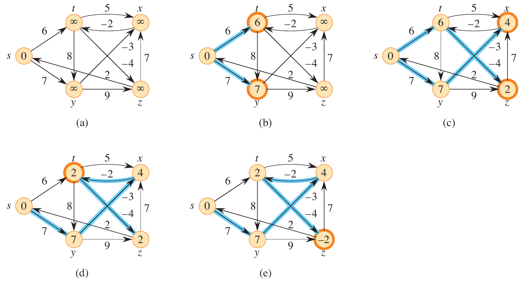
Figure 1: Step-by-step execution of Bellman-Ford on a graph with negative-weight edges (Cormen et al. 2022).
Correctness
Bellman-Ford is guaranteed to converge after \(|V| - 1\) iterations, assuming no negative-weight cycles.
Proof
The first iteration relaxes \((v_0, v_1)\). The second iteration relaxes \((v_1, v_2)\), and so on. The path-relaxation property from before implies that \(v.d = v_k.d = \delta(s, v_k) = \delta(s, v)\). If there is a negative-weight cycle, then the shortest path to \(v_k\) is not well-defined. This is verified in the final loop over the edges.
for (u, v) in G.E:
    if v.d > u.d + w(u, v):
        return False
If there exists a negative-weight cycle \(c = \langle v_0, v_1, \dots, v_k \rangle\), where \(v_0 = v_k\) that can be reached from \(s\), then
\[ \sum_{i=1}^{k} w(v_{i-1}, v_i) < 0. \]
To complete the proof by contradiction, assume that Bellman-Ford returns True. Then we would have that \(v_i.d \leq v_{i-1}.d + w(v_{i-1}, v_i)\) for \(i = 1, 2, \dots, k\) by the triangle inequality property. If we sum around the cycle, we get
\begin{align*} \sum_{i=1}^k v_i.d &\leq \sum_{i=1}^k (v_{i-1}.d + w(v_{i-1}, v_i))\\ &= \sum_{i=1}^k v_{i-1}.d + \sum_{i=1}^k w(v_{i-1}, v_i)\\ \end{align*}
Since the vertices are in a cycle, each vertex appears only once in each summation \(\sum_{i=1}^k v_{i}.d\) and \(\sum_{i=1}^k v_{i-1}.d\). Subtracting this from both sides of the inequality, we get
\[ 0 \leq \sum_{i=1}^k w(v_{i-1}, v_i). \]
This contradicts the assumption that there is a negative-weight cycle. Therefore, if Bellman-Ford returns True, then there are no negative-weight cycles.
Analysis
Using an adjacency list representation, the runtime of Bellman-Ford is \(O(V^2 + VE)\). The initialization takes \(\Theta(V)\). Each of the \(|V| - 1\) iterations over the edges takes \(\Theta(V + E)\), and the final check for negative-weight cycles takes \(\Theta(V + E)\). If the number of edges and vertices is such that the number of vertices are a lower bound on the edges, then the runtime is \(O(VE)\).
Example 22.1-1
Run Bellman-Ford on the given graph using \(z\) as the source. Then change the weight of \((z, x)\) to 4 and run it again with \(s\) as the source.
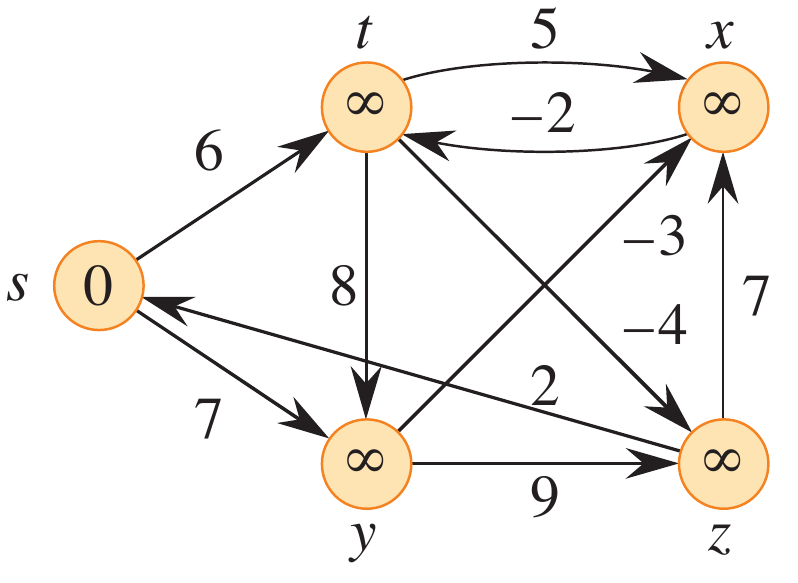
Figure 2: Figure 22.4 from (Cormen et al. 2022).
Shortest Paths on a DAG
If we are given a directed acyclic graph (DAG), we can solve the single-source shortest path problem in \(O(V + E)\) time. By definition, the graph has no cycles and thus no negative-weight cycles.
def dag_shortest_paths(G, w, s):
    initialize_single_source(G, s)
    for u in topological_sort(G):
        for v in G.adj[u]:
            relax(u, v, w)
Example
Run dag_shortest_paths on the graph given below with \(s\) as the source.
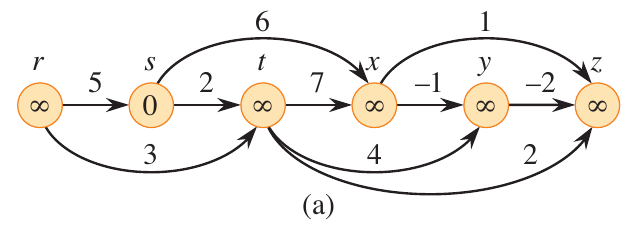
Figure 3: Figure 22.5 from (Cormen et al. 2022).
Analysis
The runtime of dag_shortest_paths is \(O(V + E)\), where \(V\) is the number of vertices and \(E\) is the number of edges. The topological sort takes \(O(V + E)\) time. Initializing the vertices takes \(O(V)\) time. The first for loop makes on iteration per vertex, and the inner loop relaxes each edge only once.
Dijkstra’s Algorithm
Dijkstra’s algorithm also solves the single-source shortest path problem on a weighted, directed graph \(G = (V,E)\) but requires nonnegative weights on all edges. It works in a breadth-first manner. A minimum priority queue is utilized to keep track of the vertices that have not been visited based on their current minimum shortest-path estimate. The algorithm works by relaxing edges, decreasing the shortest-path estimate on the weight of a shortest path from \(s\) to each vertex \(v\) until it reaches the shortest-path weight.
def dijkstra(G, w, s):
    initialize_single_source(G, s)
    S = []
    Q = G.V
    while Q:
        u = extract_min(Q)
        S.append(u)
        for v in G.adj[u]:
            prev_d = v.d
            relax(u, v, w)
            if v.d < prev_d:
                decrease_key(Q, v)
Example
A Python example of the figure below is available here.
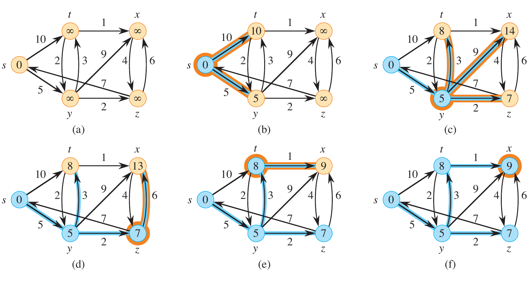
Figure 4: A step-by-step execution of Dijkstra’s algorithm on a graph with non-negative edge weights (Cormen et al. 2022).
Analysis
See Chapter 22 of Introduction to Algorithms for a detailed analysis of Dijkstra’s algorithm. Inserting the nodes and then extracting them from the queue yields \(O(V \log V)\). After extracting a node, its edges are iterated with a possible update to the queue. This takes \(O(E \log V)\). The total runtime is \(O((V + E) \log V)\).