Stereo Vision
Introduction
Binocular vision permits depth perception. It is an important part of many tasks such as robotic vision, pose estimation, and scene understanding. The goal of steropsis is to reconstruct a 3D representation of the world given correspondences between two or more cameras.
The process of computing these correspondences assumes two or more cameras with known intrinsic and extrinsic parameters. Methods exist to estimate the required transformation parameters using points based on matching image features. If some set of points which a fixed coordinate system is known, such as a calibration pattern, the problem becomes even simpler. Knowing the exact world point as it is projected in all image planes is essentially a ground truth.
Hartley and Zisserman address three primary questions when dealing with two views:
- Correspondence geometry: How does a point in one view constraint the corresponding point in a second view?
- Camera geometry: How do we determine the cameras of both views given a set of corresponding image points?
- Scene geometry: If we know the cameras and have a set of corresponding points, how can we compute the depth?
Epipolar Geometry
Epipolar geometry is the backbone of stereopsis. We will first define what epipolar geometry is, how it is used in the stereo vision problem, and the core constraint that limits our search space of point correspondences. It is defined visually below.
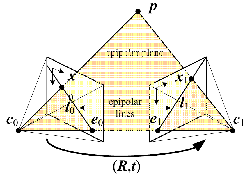
Figure 1: Overview of epipolar geometry for stereopsis (Source: Szeliski).
Consider the point \(\mathbf{p}\) whose projection is \(\mathbf{x}_0\) with respect to camera \(\mathbf{c}_0\) and \(\mathbf{x}_1\) with respect to camera \(\mathbf{c}_1\). All 5 of these points lie on the epipolar plane. Additionally, points \(\mathbf{e}_0\) and \(\mathbf{e}_1\) lie on the line defined by \(\mathbf{c}_0\) and \(\mathbf{c}_1\) as it intersects the image plane of each camera, respectively. These are called the epipoles. These are also the projections of the other camera centers.
Fundamental to establishing the correspondences between the two cameras is the epipolar constraint. If \(\mathbf{x}_0\) and \(\mathbf{x}_1\) represent projections of the same point, then \(\mathbf{x}_1\) must like on the epipolar line \(l_1\) associated with \(\mathbf{x}_0\) and vice versa.
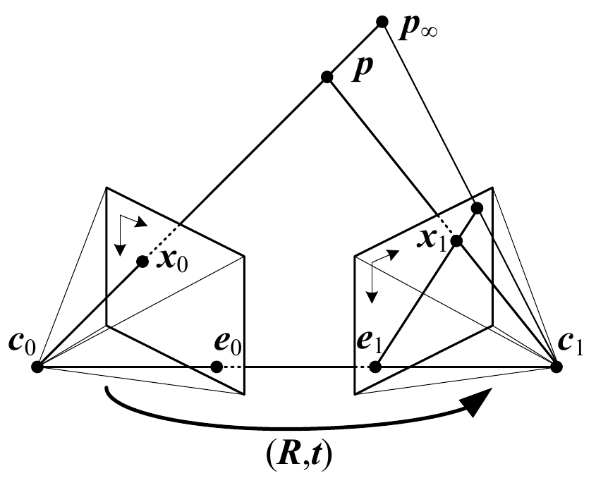
Figure 2: The epipolar constraint restricts the search space for matching correspondences. (Source: Szeliski)
As seen in the figure above, potentional matches for \(\mathbf{x}_0\) must lie on the epipolar line defined by \(\mathbf{e}_1\) and \(\mathbf{x}_1\).
Our goal is to compute translation \(\mathbf{t}\) and rotation \(R\). To find these, we start by mathematically defining the epipolar constraint. The epipolar plane is defined by the lines \(\overrightarrow{\mathbf{c}_0 \mathbf{p}}\), \(\overrightarrow{\mathbf{c}_1 \mathbf{p}}\), and \(\overrightarrow{\mathbf{c}_0 \mathbf{c}_1}\). This can be written as
\[ \overrightarrow{\mathbf{c}_0 \mathbf{p}} \cdot [\overrightarrow{\mathbf{c}_0 \mathbf{c}_1} \times \overrightarrow{\mathbf{c}_1 \mathbf{p}}] = 0. \]
We do not know \(\mathbf{p}\), but we do have \(\mathbf{x}_0\) and \(\mathbf{x}_1\), the projections of \(\mathbf{p}\) onto the image plane of each respective camera. Assuming that both camera are calibrated, we have a set of known intrinsic matrices \(\mathbf{K}_j\).
Although we do not have the exact \(z\) value of the point, we do know the point with respect to the camera calculcated as
\[ \mathbf{p}_0 = d_0 \hat{\mathbf{x}}_0, \]
where
\[ \hat{\mathbf{x}}_0 = \mathbf{K}_0^{-1} \mathbf{x}_0. \]
The relationship between points \(\mathbf{p}_0\) and \(\mathbf{p}_1\) is
\[ d_1 \hat{\mathbf{x}}_1 = R(d_0 \hat{\mathbf{x}}_0) + \mathbf{t}, \]
where \(R\) is a rotation matrix and \(\mathbf{t}\) is an offset vector. These are the parameters that are solved from stereo calibration.
Essential Matrix
Given the definitions and constraints above, we can now discuss the essential matrix, which contains the rotation and translation parameters that map the point in camera 1 with the corresponding point in camera 2. The epipolar constraint is simplified in this case:
\[ \hat{\mathbf{x}}_0 \cdot (\mathbf{t} \times \hat{\mathbf{x}}_0) = 0. \]
With this constraint, we can set up the equation to solve for the rotation and translation parameters. Ultimately, we are attempting to solve the following equation:
\[ \hat{\mathbf{x}}_1 = R \hat{\mathbf{x}}_0 + \mathbf{t}. \]
Since the vectors \(\hat{\mathbf{x}}_0\), \(\hat{\mathbf{x}}_1\), and \(\mathbf{t}\) are coplanar, the plane can be represented by a normal vector. That is, the vector that is orthogonal to all points in the plane. Such a vector can be calculated by taking the cross product of both sides of the above equation with \(\mathbf{t}\):
\[ [\mathbf{t}]_{\times} \hat{\mathbf{x}}_1 = [\mathbf{t}]_{\times} R \hat{\mathbf{x}}_0 + [\mathbf{t}]_{\times} \mathbf{t}, \]
where
\[ [\mathbf{t}]_{\times}=\begin{bmatrix} 0 & -t_z & t_y\\ t_z & 0 & -t_x\\ -t_y & t_x & 0 \end{bmatrix}. \]
It is true that, since the normal vector is orthogonal to \(\hat{\mathbf{x}}_0\), \(\hat{\mathbf{x}}_1\), and \(\mathbf{t}\), taking the dot product of any of these vectors and the normal vector yields 0:
\[ \hat{\mathbf{x}}_1^T [\mathbf{t}]_{\times} \hat{\mathbf{x}}_1 = \hat{\mathbf{x}}_1^T [\mathbf{t}]_{\times} R \hat{\mathbf{x}}_0 = 0. \]
We have now established the epipolar constraint in terms of the rotation matrix \(R\) and translation \(\mathbf{t}\). These are the parameters that relate the points between both cameras. This constraint is more compactly written as
\[ \hat{\mathbf{x}}_1^T E \hat{\mathbf{x}}_0 = 0, \]
where
\[ E = [\mathbf{t}]_{\times}R. \]
\(E\) is called the essential matrix which relates the projected points between the two cameras. Once we have the essential matrix, we can compute \([\mathbf{t}]_{\times}\) and \(R\).
The decomposition of \(E\) into \([\mathbf{t}]_{\times}\) and \(R\) can be found using singular value decomposition (SVD). See Hartley and Zisserman (9.6.1) for more details.
Calibration with Known Intrinsic Parameters and World Points
We first look at the simplest case of stereo calibration. The intrinsic parameters of both cameras have been computed using a standard calibration technique. Additionally, we have a fixed calibration pattern used to establish a correspondence between the world points and the points with respect to each camera.
Given \(N\) measured correspondences \(\{(\mathbf{x}_{i0}, \mathbf{x}_{i1})\}\), we can form a linear system with equations of the form
\begin{alignat*}{3} x_{i0}x_{i1}e_{00} & {}+{} & y_{i0}x_{i1}e_{01} & {}+{} & x_{i1}e_{02} & {}+{} &\\ x_{i0}y_{i1}e_{10} & {}+{} & y_{i0}y_{i1}e_{11} & {}+{} & y_{i1}e_{12} & {}+{} &\\ x_{i0}e_{20} & {}+{} & y_{i0}e_{21} & {}+{} & e_{22} & {}={} & 0 \end{alignat*}
Given at least 8 equations corresponding to the 8 unknowns of \(E\), we can use SVD to solve for \(E\).
\[ E = [\mathbf{t}]_{\times}R = \mathbf{U \Sigma V^T} = \begin{bmatrix} \mathbf{u}_0 & \mathbf{u}_1 & \mathbf{t} \end{bmatrix}\begin{bmatrix} 1 & 0 & 0\\ 0 & 1 & 0\\ 0 & 0 & 1\\ \end{bmatrix}\begin{bmatrix} \mathbf{v}_0^T\\ \mathbf{v}_1^T\\ \mathbf{v}_2^T\\ \end{bmatrix} \]
Estimating Depth
Given the intrinsic parameters and parameters relating both calibrated cameras, we can estimate the depth of a point that is seen by both cameras.
We know that \(\mathbf{x}_0 = K_0 \hat{\mathbf{x}}_0\) and \(\mathbf{x}_1 = K_1 \hat{\mathbf{x}}_1\). With the stereo calibration complete, we also know \(A = [R\quad \mathbf{t}]\) and
\[ \hat{\mathbf{x}}_0 = A\hat{\mathbf{x}}_1. \]
Plugging into the projection equation for the first camera yields
\[ \mathbf{x}_0 = K_0 A\hat{\mathbf{x}}_1. \]
Our knowns are \(\mathbf{x}_0, \mathbf{x}_1, K_0, K_1, \text{ and } A\). The only unknown is \(\hat{\mathbf{x}}_1\).
We are left with 2 equations
\begin{align*} \mathbf{x}_0 &= K_0 A\hat{\mathbf{x}}_1\\ \mathbf{x}_1 &= K_1 \hat{\mathbf{x}}_1. \end{align*}
If we let \(P = K_0 A\), we write the \(\mathbf{x}_0 = \begin{bmatrix}u_1\\v_1\\1\end{bmatrix}\) and
\begin{equation*} \begin{bmatrix} u_1\\ v_1\\ 1 \end{bmatrix}=\begin{bmatrix} p_{11} & p_{12} & p_{13} & p_{14}\\ p_{21} & p_{22} & p_{23} & p_{24}\\ p_{31} & p_{32} & p_{33} & p_{34}\\ \end{bmatrix}\begin{bmatrix} X\\ Y\\ Z\\ W \end{bmatrix}. \end{equation*}
This gives two equations for \(x_1\) and \(y_1\), the measured 2D feature locations:
\begin{align*} x_1 &= \frac{p_{11}X + p_{12}Y + p_{13}Z + p_{14}W}{p_{31}X + p_{32}Y + p_{33}Z + p_{34}W}\\ y_1 &= \frac{p_{21}X + p_{22}Y + p_{23}Z + p_{24}W}{p_{31}X + p_{32}Y + p_{33}Z + p_{34}W}. \end{align*}
Multiplying both equations by the denominator yields a set of equations that can be solved via linear least squares or SVD.