Topological Sort
Topological Sort
A topological sort of a directed acyclic graph \(G = (V, E)\) is a linear ordering of all its vertices such that for every directed edge \((u, v) \in E\), vertex \(u\) comes before vertex \(v\) in the ordering.
The process itself can be described simply:
- Call \(\text{DFS}(G)\) to compute the finishing times for each vertex \(v\).
- As each vertex is finished, insert it onto the front of a linked list.
- Return the linked list of vertices.
The entire call takes \(\Theta(V + E)\) since DFS\((G)\) takes \(\Theta(V + E)\) time. Inserting each vertex onto the front of the list can be done in constant time.
Lemma
A directed graph \(G\) is acyclic if and only if a DFS of \(G\) yields no back edges – an edge \((u, v)\) such that \(v\) is an ancestor of \(u\) in the DFS forest.
Proof
The proof is by contradiction: if a back edge exists, then there is a cycle in the graph.
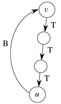
Figure 1: A back edge between edges (u) and (v) (Cormen et al. 2022).
Suppose there is a back edge \((u, v)\) as shown in the figure above. In this case, \(v\) is an ancestor of \(u\) in the depth-first forest. There is a path \(v \leadsto u\), so \(v \leadsto u \rightarrow v\) is a cycle.
In the other direction, suppose that \(G\) contains a cycle \(c\). Let \(v\) be the first vertex discovered in \(c\), and let \((u, v)\) be the preceding edge in \(c\). At time \(v.d\), vertices of \(c\) form a white path \(v \leadsto u\). Since \(u\) is a descendant of \(v\), \((u, v)\) is a back edge. \(\blacksquare\)
Theorem
The topological sort algorithm produces a topological sort of a directed acyclic graph.
Proof
Run a DFS on the graph \(G\) to determine finish times for its vertices. For any pair of vertices \((u, v)\), if \(G\) contains an edge from \(u\) to \(v\), then \(v.f < u.f\). (Review DFS).
Example
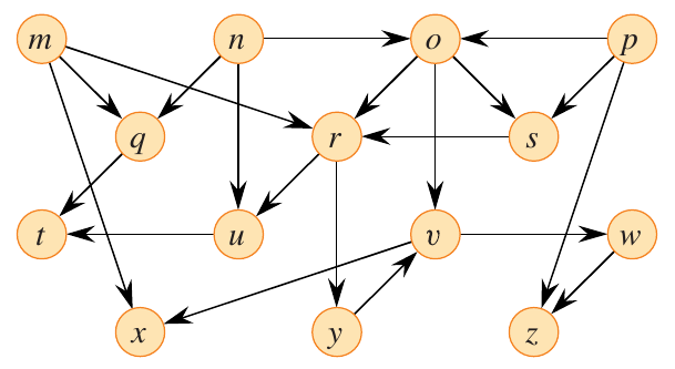
Figure 2: DAG for topological sorting. Figure 20.8 from (Cormen et al. 2022).
Strongly Connected Components
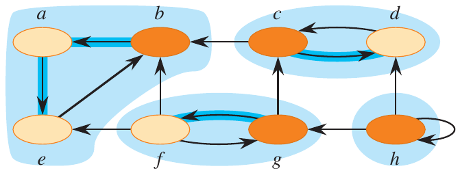
Figure 3: Strongly connected components of a directed graph (Cormen et al. 2022).
A strongly connected component of a directed graph \(G\) is a maximal set of vertices such that for every pair of vertices \(u\) and \(v\) in the set, there is a path from \(u\) to \(v\) and a path from \(v\) to \(u\). The algorithm goes as follows:
- Call \(\text{DFS}(G)\) to compute the finishing times for each vertex \(v\).
- Compute the transpose of \(G\).
- Call \(\text{DFS}(G^T)\), but in the main loop of DFS, consider the vertices in order of decreasing finishing times.
- Output the vertices of each tree in the depth-first forest as a separate strongly connected component.
The transpose of a graph \(G^T\) is the graph \(G\) with all edges reversed.
\begin{align*} G^T &= (V, E^T) \\ E^T &= \{(v, u) \mid (u, v) \in E\} \end{align*}
Component Graphs
The resulting component graph is a directed graph \(G_{SCC} = (V_{SCC}, E_{SCC})\) where each vertex represents a strongly connected component of the original graph \(G\). There is an edge \((C_i, C_j)\) in \(G_{SCC}\) if there is a vertex \(u \in C_i\) and a vertex \(v \in C_j\) such that \((u, v) \in E\). The component graph of the DAG from above is shown below.
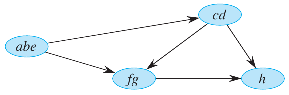
Figure 4: Component graph of the DAG from above (Cormen et al. 2022).
Lemma
The component graph \(G^{SCC}\) is a directed acyclic graph. Let \(C\) and \(C’\) be distinct strongly connected components in \(G\), where \(u, v \in C\) and \(u’, v’ \in C’\), and suppose there is a path \(u \leadsto u’\) in \(G\). Then there cannot also be a path \(v’ \leadsto v\) in \(G\).
Proof
Suppose there is a path \(v’ \leadsto v\) in \(G\). This implies there are paths \(u \leadsto u’ \leadsto v’\) and \(v’ \leadsto v \leadsto u\). If this were possible, then \(u\) and \(v’\) are reachable from each other, which contradicts the assumption that \(C\) and \(C’\) are distinct strongly connected components. \(\blacksquare\)
Example
Finishing Times
The previous and following lemmas establish, given the algorithm presented above, the rules of the finishing times of strongly connected components. These are used to prove the correctness of the algorithm.
Lemma
Let \(C\) and \(C’\) be strongly connected components in a directed graph \(G\). If there is an edge \((u, v) \in E\) such that \(u \in C\) and \(v \in C’\), then \(f( C) > f(C’)\).
Proof
There are two cases to consider depending on which strongly connected component had the first discovered vertex during the first DFS call.
Case 1
- If \(d( C) < d(C’)\), let \(x\) be the first vertex discovered in \(C\). At time \(x.d\), the time of discovery, all vertices in \(C\) and \(C’\) are white. Thus, there exists paths of white vertices from \(x\) to all vertices in \(C\) and \(C’\).
- By the white-path theorem, all vertices in \(C\) and \(C’\) are descendants of \(x\) in the depth-first tree.
- By the parenthesis theorem, \(x.f = f( C) > f(C’)\).
Case 2
- If \(d( C) > d(C’)\), let \(y\) be the first vertex discovered in \(C’\). At time \(y.d\), all vertices in \(C\) and \(C’\) are white. Thus, there exists paths of white vertices from \(y\) to all vertices in \(C’\). All vertices in \(C’\) become descendants of \(y\). Again, \(y.f = f(C’)\).
- At time \(y.d\), all vertices in \(C\) are also white.
- Since there is an edge \((u, v)\), where \(u \in C\) and \(u’ \in C’\), we cannot have a path from \(C’\) to \(C\).
- No vertex in \(C\) is reachable from \(y\).
- Therefore, at time \(y.f\), all vertices in \(C\) are white.
- Therefore, for all \(w \in C, w.f > y.f\), which implies that \(f( C) > f(C’)\). \(\blacksquare\)
Corollary
Let \(C\) and \(C’\) be distinct strongly connected components in \(G\). Suppose there is an edge \((u, v) \in E^T\), where \(u \in C\) and \(v \in C’\). Then \(f( C) < f(C’)\).
Proof
- \((u, v) \in E^T \implies (v, u) \in E\)
- Since strongly connected components of \(G\) and \(G^T\) are the same, \(f(C’) > f( C)\).
Correctness
Now we can combine the previous results to prove the correctness of the algorithm.
Corollary
Let \(C\) and \(C’\) be distinct strongly connected components in \(G\), and suppose that \(f( C) > f(C’)\). Then there cannot be an edge from \(C\) to \(C’\) in \(G^T\).
Proof
When we perform the second DFS call, on \(G^T\), it starts with the component \(C\) such that \(f( C)\) is the maximum. This call starts from some \(x \in C\) and explores all vertices in \(C\). The corollary says that since \(f( C) > f(C’)\), there cannot be an edge from \(C\) to \(C’\) in \(G^T\). Therefore, DFS will visit only vertices in \(C\). This means that the depth-first tree rooted at \(x\) will contain only vertices in \(C\).
The next root chosen is in \(C’\) such that \(f(C’)\) is maximum over all strongly connected components other than \(C\). DFS visits all vertices in \(C’\), but the only edges out of \(C’\) go to \(C\), which have already been visited. Therefore, the only tree edges will be to vertices in \(C’\).
As this process continues, we can observe that each root chosen for the second DFS can reach only
- vertices in its own strongly connected component, and
- vertices in strongly connected components already visited in the second DFS.
Application: Recommender Graphs
A recommender graph is a directed graph where each vertex represents an item and each edge represents a transition between the items based on the context of the data. For example, in a movie recommender graph, each vertex represents a movie, and an edge from \(u\) to \(v\) indicates that users typically transitioned from watching movie \(u\) to watching movie \(v\). The weight of such an edge could be the number of users who made the transition or the average rating improvement when moving from \(u\) to \(v\) (Lamprecht, Strohmaier, and Helic 2017).
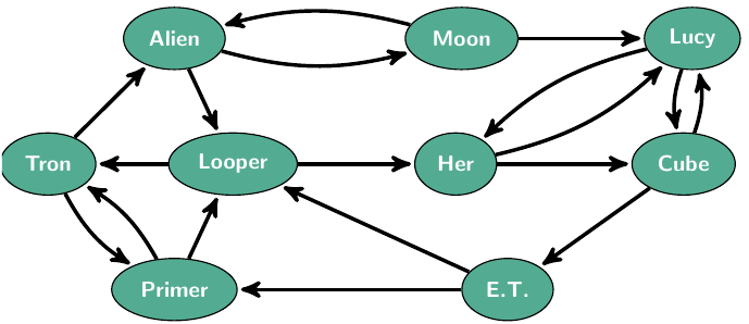
Figure 5: A recommender graph (Lamprecht, Strohmaier, and Helic 2017).
In such a graph, strongly connected components can be used to identify groups of items that are closely related. Based on this information, a recommender system can suggest items that are similar to the ones a user has already interacted with. If the edges contained information such as improvement of ratings, the recommendation system could suggest items that are likely to be enjoyed by the user.
Identifying such a strongly connected component can also provide insights into the structure of the data. Given the current recommender graph, it is possible that the strongly connected component related to a particular sub-genre of movies is small, leading to a cycle of recommendations within that sub-genre. This discovery would prompt the recommender system to suggest items from other genres to provide a more diverse set of recommendations.